3. Estimating the income density function

Eric Graf and Yves Tillé

Previous | Next

In a design-based approach with a finite population, inference is made in relation to the sampling design $P(S)$  used to select a sample  $S$ from a finite population  $U$ of size  $N$ . In this approach, only the sample inclusion indicators are random; all other quantities are fixed. The population income distribution function is then a step function: $F_y\left(x\right)={\displaystyle {\sum }_{k\in U}{1}_{y_k\le x}}/N$ , and its derivative, the density function, does not exist due to discontinuities. If a model-based approach with a super-population model to justify the income density function term is not desired, then the distribution function must be artificially smoothed to make it differentiable. Therefore, our use of “density function” is not quite correct. For purposes of smoothing, Deville (2000) and Osier (2009) suggest using Gaussian kernel estimation to estimate the income density function:

$$\begin{array}{lllll}K\left(u\right)\hfill & =\hfill & \frac{1}{h\sqrt{2\pi }}{e}^{-u^2/2}\mathrm{,}u=\frac{x-y_k}{h}\hfill & \hfill & \hfill \\ {\widehat{f}}_1\left(x\right)\hfill & =\hfill & \frac{1}{\widehat{N}}{\displaystyle \sum _{k\in S}}{w}_{k}K\left(\frac{x-y_k}{h}\right)\hfill & \hfill & \left(3.1\right)\hfill \\ \hfill & =\hfill & \frac{1}{h\sqrt{2\pi }}\frac{1}{\widehat{N}}{\displaystyle \sum _{k\in S}}{w}_k\exp \left[-\frac{{\left(x-y_k\right)}^2}{2h^2}\right]\hfill & \hfill & \hfill \end{array}$$

where $h$  is the bandwidth that Osier estimates using $\widehat{h}=\widehat{\sigma }{\widehat{N}}^{-\text{0}\text{.2}}$  and $\widehat{\sigma }$  is the estimated standard deviation of the empirical income distribution:

$$\widehat{\sigma }=\sqrt{\frac{{\displaystyle {\sum }_{k\in S}{w}_k{y}_k^2}}{\widehat{N}}-{\left(\frac{{\displaystyle {\sum }_{k\in S}{w}_k{y}_k}}{\widehat{N}}\right)}^2}=\sqrt{\frac{{\displaystyle {\sum }_{k\in S}{w}_k{y}_k^2}}{\widehat{N}}-{\overline{y}}_w^2}\mathrm{.}$$

Note that this estimate of $\sigma$  is not robust, since it is very sensitive to the extreme values of $y.$  Income data often have a distribution tail extending to the right with values that may be extremely high; these are “representative outliers” as defined by Chambers (1986) and Hulliger (1999). As the simulations in Section 4 will show, this can generate a strong bias in the variance estimates. Verma and Betti (2011) also use kernel estimation, recalling that Silverman (1986) states that the choice of kernel is not critical to ensure that $\widehat{f}\left(y\right)$  converges toward $f\left(y\right),$  but the choice of bandwidth is. They use a value recommended by Silverman for distributions with a positive skewness coefficient, $h=\text{0}\text{.79(}{\widehat{Q}}_{75}-{\widehat{Q}}_{25}){\widehat{N}}^{-\text{0}\text{.2}}.$  In their findings, they point out that the linearization method may be problematic because of irregularities in the empirical density function. They also state that these problems are all the more cause for concern because survey data often contain groups of observations with the same value (due to rounding or range questions), which can make estimating the density more complicated. The rest of this article describes the solutions we are proposing to reduce bias in variance estimates.

3.1 Using the logarithm

One solution that produces very good results, as shown below, is simply to use the logarithm to estimate the density of $x.$  If $v=\log \left(x+a\right),$  where $x$  is the income and $a$  is a positive real number equals to, say, $\left(\left|{{\displaystyle \min }}_k(y_k)\right|+1\right)$  where there may be negative or zero incomes (ignoring that $a$  would be estimated), then

$$F_v\left(v\right)=P\left(\mathcal{V}\le v\right)=P\left(\log \left(\mathcal{Y}+a\right)\le v\right)=P\left(\mathcal{Y}\le e^v-a\right)=F_y\left(e^v-a\right)\mathrm{,}$$

where $\mathcal{V}$  and $\mathcal{Y}$  would be random variables. Therefore,

$$f_v\left(v\right)=\frac{d{F}_v\left(v\right)}{dv}=\frac{d{F}_y\left(e^v-a\right)}{dv}=f_y\left(e^v-a\right)e^v\mathrm{.}$$

That is, $f_v\left(v\right)=f_y\left(x\right)\left(x+a\right),$  which gives us the following estimator for the density of $x:$

$${\widehat{f}}_2\left(x\right)=\frac{{\widehat{f}}_v\left(v\right)}{x+a}=\frac{{\widehat{f}}_y\left(\log \left(x+a\right)\right)}{x+a}\mathrm{.}\left(3.2\right)$$

The estimated density at $x$  for $\mathcal{Y}$  can therefore be determined by estimating the density of the logarithm of the variable divided by the value of the variable at a given point. This property is valid for finite populations. Using the logarithm has the advantage of reducing the leveraging effect of large income values in the kernel density approximation calculation. Simulations show that this simple method significantly reduces bias.

3.2 Nearest neighbour with minimum bandwidth

Deville (2000) outlines another density estimation method that is a “nearest neighbour” method (see Silverman 1986) using the kernel

$$K_D\left(u\right)=\{\begin{array}{ll}\frac{1}{b-a}\hfill & \text{if}a\le u<b\hfill \\ 0\hfill & \text{otherwise}\mathrm{,}\hfill \end{array}\mathrm{,}$$

where $u=y_k$  and the choice of $a$  and $b,$  with $x\in \left[a,b\right],$  is to be determined and could depend on $x.$  The distance $\left(b-a\right)$  represents the bandwidth $h.$  The density estimate would therefore be

$$\begin{array}{lllll}{\widehat{f}}_D\left(x\mathrm{,}a\mathrm{,}b\right)\hfill & =\hfill & \frac{1}{\widehat{N}}{\displaystyle \sum _{k\in S}}{K}_D\left(y_k\right)\hfill & \hfill & \hfill \\ \hfill & =\hfill & \frac{1}{\widehat{N}}{\displaystyle \sum _{k\in S}}{w}_k\frac{1}{b-a}{1}_{y_k\in \left[a\mathrm{,}b\right[}\hfill & \hfill & \left(3.3\right)\hfill \\ \hfill & =\hfill & \frac{{\widehat{F}}_y\left(b\right)-{\widehat{F}}_y\left(a\right)}{b-a}\mathrm{,}x\in \left[a\mathrm{,}b\right[\hfill & \hfill & \hfill \end{array}$$

where ${\widehat{F}}_y\left(x\right)={\displaystyle {\sum }_{k\in S}{w}_k{1}_{y_k\le x}/\widehat{N}}.$

Note that the density estimate (3.3) is not a continuous function and would not be suitable for estimating density values at the end tails of the distribution. Since our work relies little on distribution tails, we shall consider this approach as an option.

Our second proposal for estimating the density of $x$  is based on the idea above. It is a nearest neighbour method, but also imposes a minimum bandwidth. Specifically, our method requires the use of at least $p$ observations nearest to point  $x$ with minimum bandwidth $h(p)\ge h_{opt}$ where

$$h_{\text{opt}}=\frac{\text{0}\text{.9}\min (\widehat{\sigma }\mathrm{,}{\widehat{Q}}_{75}-{\widehat{Q}}_{25})}{\text{1}\text{.34}\sqrt[5]{\widehat{N}}}$$

is the rule of thumb (Silverman 1986) for determining the bandwidth. This is also the default bandwidth value in the R function density. This solution is more robust than (3.1) and avoids the problems that arise when a number of values $y_k$  are very close to each other, which is often the case because the individuals interviewed tend to round their income.

As the values $y_k,$   $k=1,\mathrm{...},n,$  are assumed to be ordered by rank, the width $h\left(p\right)$  of the window around $x$  is initially determined by the $p$  nearest observations, where $p\ll n.$  In the simulations discussed in the next section, after various trials, $p$  was initially set at 30. The density of $x$  is imputed to be the estimated density at the nearest observed point $y_j$  that is less than or equal to $x,$  that is, $j=\max \left(k|y_k\le x\right),$   $k=1,\mathrm{...},n.$  The bandwidth at $x$  in fact depends on the $p_j$  nearest observations around $y_j,$  with $p_j\ge p,$  which will be denoted $h\left(p_j\right)$  in the rest of this article. The density is therefore estimated only at observed points, with no smoothing or interpolation between the values $\widehat{f}\left(y_j\right).$  The algorithm for estimating $\widehat{f}\left(y_j\right)$  is as follows (see also Figure 3.1):

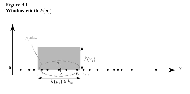
1.   The initial width of the window around point  $y_j,$ where $p_j=p,$ is defined as

$$\begin{array}{llll}h\left(p_j\right)=\frac{y_u+y_{u+1}}{2}-\frac{y_{\ell }+y_{\ell -1}}{2};\hfill & u\hfill & =\hfill & \{\begin{array}{ll}j+p_j/2-1\hfill & \text{if}{p}_j\text{is}\text{even}\hfill \\ j+\lfloor p_j/2\rfloor \hfill & \text{if}{p}_j\text{is}\text{odd}\hfill \end{array}\hfill \\ \hfill & \ell \hfill & =\hfill & j-\lfloor p_j/2\rfloor \mathrm{.}\hfill \end{array}$$

2.   If the width of the resulting window $h(p_j)$  is less than $h_{opt}$, increment the two bounds:

upper bound: $u\to u+1,$ as long as $u<n,$

lower bound: $l\to l-1,$  as long as $l\text{>}1,$

which implies that $p_j\to p_j+2,$  unless $u=n$  or $l=1,$  in which case there is no longer the same number of points on each side of $y_j.$

3.   Repeat step 2 until $h\left(p_j\right)\ge h_{\text{opt}}.$

4.   The estimated density at $x$  can then be written as

$$\widehat{f}\left(x\right)=\widehat{f}\left(y_j\right)=\{\begin{array}{ll}\frac{p_j}{nh\left(p_j\right)}\hfill & \text{without weighting}\mathrm{,}\hfill \\ \frac{{\displaystyle \sum _{p_{j}closestto{y}_j}}{w}_j^{\text{std}}}{nh\left(p_j\right)}\hfill & \text{with weighting}\mathrm{,}\hfill \end{array}$$

with standardized weights $w_k^{\text{std}}=w_k/\overline{w},$ $k=1,\mathrm{...},n.$

The number of observations $p_j$  used in the calculation may vary, and it depends on the local curvature of the empirical distribution function. The condition $h(p_j)\ge h_{opt}$  guarantees a minimum window width in places where numerous observations would be concentrated over a small interval. The procedure is made even more solid by combining this approach with the preceding approach, that is, by estimating the density of the logarithm of the variable divided by its (non-logarithmic) value:

$${\widehat{f}}_3\left(x\right)=\frac{\widehat{f}\left(\text{log}\left(x+a\right)\right)}{x+a}\mathrm{.}\left(3.4\right)$$

3.3 Robustness of the linearized variable

As stated above, for the median or for other quantiles, Croux (1998) points out that the empirical influence function or the linearized variable estimated using the sample is not as robust as it appears to be, even if the density function is known. We confirmed this for the EU-SILC data used in the model simulations with a Generalized Beta distribution of the second kind (GB2) by means of the R function profml.gb2 (Graf and Nedyalkova 2011). For small samples $\left(n\le 100\right),$  the potential bias of the linedarized variable resulting from too many outliers may also bias the variance estimate calculated using the linearized variable. For larger samples $\left(n\ge 1,000\right),$  a maximum relative bias in the variance estimated using the empirical versus theoretical linearized variable may reach 5%. However, it is below the percentage in absolute terms three times out of four.

Previous | Next