4 An example based on the Iris flowers dataset

Marco Ballin and Giulio Barcaroli

To show how to apply the algorithm for finding the optimal stratification, the well known Iris flowers dataset can be considered. This dataset consists of a total of 150 observations, equally distributed by the three species of Iris flowers (setosa, virginica and versicolor). Four features are measured for each observation (i.e., the length and the width of sepal and petal, in centimetres).

We will consider this dataset as a possible sampling frame from which to draw a sample, under a stratified design, in order to estimate two target variables:

$Y_{1}$ : Petal.Length;
$Y_{2}$ : Petal.Width.

For sake of simplicity, we suppose there are only two auxiliary variables available in the frame:

$X_{1}$ : Sepal.Length;
$X_{2}$ : Species.

While the second auxiliary variable is categorical, the first one is continuous, and needs to be transformed into a categorical ordered variable. To this aim, we make use of the $k $ means univariate clustering method (Hartigan and Wong 1979), obtaining the following ranges: [4.3; 5.5], (5.5; 6.5], (6.5; 7.9].

The Cartesian product of the two auxiliary variables should produce $3 \times 3 = 9$ different strata. Actually, one of these contains no units, the one related to Species $=$ "setosa� and Sepal.Length $\in$ (6.5; 7.9]. So the one reported in table 4.1 will be considered as the initial atomic stratification.

Table 4.1
Information concerning atomic strata
Table summary
This table displays information concerning atomic strata. The information is grouped by stratum, X ₁ = Sepal.Length, X ₂ = Species, N, Y ₁ = Petal.Length, Y ₁ = Petal.Width, Cost (appearing as column headers).
stratum	X ₁ = Sepal.Length	X ₂ = Species	N	Y ₁ = Petal.Length		Y ₁ = Petal.Width		Cost
stratum	X ₁ = Sepal.Length	X ₂ = Species	N	Mean	Standard deviation	Mean	Standard deviation	Cost
1	[4.3; 5.5] (1)	Setosa (1)	45	1.47	0.17	0.24	0.11	1
2	[4.3; 5.5] (1)	Versicora (2)	6	3.58	0.49	1.17	0.21	1
3	[4.3; 5.5] (1)	Virginica (3)	1	4.50	0.00	1.70	0.00	1
4	[5.5; 6.5] (2)	Setosa (1)	5	1.42	0.17	0.26	0.08	1
5	[5.5; 6.5] (2)	Versicora (2)	35	4.27	0.37	1.32	0.19	1
6	[5.5; 6.5] (2)	Virginica (3)	23	5.23	0.32	1.95	0.29	1
7	[6.5; 7.9] (3)	Versicora (2)	9	4.68	0.19	1.46	0.11	1
8	[6.5; 7.9] (3)	Virginica (3)	26	5.88	0.49	2.11	0.23	1

For sake of simplicity, we assume that the fixed cost $C_{0}$ is null, and all $C_{h}$ are set equal to 1: by so doing, the cost of a solution coincides with the sum of sampling units allocated in the strata, i.e., with the total sample size $(C = n = \sum_{h = 1}^{H} n_{h}) .$

We set as precision constraints to the estimates of both target variables an upper limit of 0.05 (5%) to their expected coefficient of variation.

Finally, we set a minimum number of units to be selected in each stratum equal to 2 (the minimum required in order to calculate sampling variance).

Under these assumptions, and using the atomic stratification, the Bethel algorithm solves the optimal allocation problem by defining a minimum sample size of 17 units, with an allocation vector $a = (2, 2, 1, 2, 3, 3, 2, 2) .$

If we proceed to partition the set of atomic strata, the resulting number of all possible stratifications (given by the Bell formula) is $B_{8} =$ 4,140. This number is such that we can afford to enumerate all partitions of atomic strata, and for each of them we are able to calculate the minimum sample size by applying the Bethel algorithm (to enumerate all the partitions in this example, we made use of the function setparts(), contained in the R package partitions (Hankin 2011)).

The range of sample sizes steps from a minimum of 11 to a maximum of 78 (this latter corresponds to the "no stratification solution�) (see figure 4.1).

Description for figure 4.1

Figure 4.1 Space of partitions

We notice that the minimum value $(n = 11)$ that has been found is considerably lower than the one calculated in correspondence with the atomic stratification $(n = 17) .$ This minimum value characterizes only 8 partitions out of 4,140.

Now, the genetic algorithm is applied in order to evaluate its capability to find the optimal solution (or at least one that is not far from it), without being obliged to explore all solutions, but only a strict subset of them.

Step 0: Creation of the initial generation

First, we set $U = 8$ (we can accept a number of final strata that is equal to the number of atomic strata, so $U = K$ ). The generation size parameter pop is set equal to 10. So, an initial set containing 10 different individuals (stratifications) is generated. Each of them is represented by a vector of 8 elements, i.e., the number of different atomic strata. An individual $v = (1, 2, 3, 4, 5, 6, 7, 8)$ or, equivalently, $v = (3, 6, 4, 2, 1, 8, 7, 5)$ corresponds to the most detailed stratification (as all strata are labelled with different labels), while $v = (1, 1, 1, 1, 1, 1, 1, 1)$ or equivalently $v = (4, 4, 4, 4, 4, 4, 4, 4)$ corresponds to "null stratification� (as atomic strata are labelled with identical labels).

Step 1: Evaluation of fitness for each individual in the generation

To each one of the 10 individuals in the current generation, the Bethel algorithm is applied in order to find the cost of the sample required to comply with fixed precision constraints.

To do this, first of all related strata and information are calculated for each individual. For example, for a generated individual $v = (4, 1, 1, 4, 8, 7, 8, 1)$ the information is derived by the one available from atomic strata, by applying (3.1) and (3.2) (see table 4.2).

Table 4.2
Information concerning generated aggregated strata
Table summary
This table displays information concerning generated aggregated strata. The information is grouped by Aggregated stratum, Original atomic strata, ( X ₁, X ₂), N, Y ₁, Y ₂ (appearing as column headers).
Aggregated stratum	Original atomic strata	( X ₁, X ₂)	N	Y ₁		Y ₂
Aggregated stratum	Original atomic strata	( X ₁, X ₂)	N	Mean	Standard deviation	Mean	Standard deviation
1	2,3,8	(1,2) or (1,3) or (3,3)	33	5.41	1.01	1.92	0.44
2	1,4	(1,1) or (2,1)	50	1.46	0.17	0.25	0.10
3	6	(2,3)	23	5.23	0.31	1.95	0.28
4	5,7	(2,2) or (3,2)	44	4.35	0.37	1.35	0.18

The fitness of this individual is measured by the corresponding required sample size, that results to be 14, with an allocation vector $a = (6, 2, 3, 3) .$

All individuals are sorted accordingly with their performance: the individual in the first position is the one supporting the minimum sample size, the 10^th individual is the one requiring the maximum sample size.

Step 2: Breeding a new generation

By setting the elitism parameter to 20% (a common default value) we always take the best 2 individuals in the current generation and directly move them to the next generation, without any change of their genome.

Then, we proceed in generating new individuals in the following way:

we select couples of individuals of the current generation with probability proportional to their fitness: for instance, assume to select $v_{k} = (1, 1, 3, 4, 3, 2, 2, 2)$ and $v_{j} = (2, 2, 2, 2, 2, 1, 1, 1);$
a crossover point is randomly generated, i.e., an integer internal to the interval $[1, 8] :$ suppose to set it equal to 3;
the crossover is performed by assigning to the child the first three elements of parent $v_{k}$ and the last five elements of parent $v_{j},$ obtaining in this way $v_{new} = (1, 1, 3, 2, 2, 1, 1, 1);$
having set a mutation rate parameter equal to 0.05, for each element of the child a random number is generated in the interval $[0, 1] :$ if it is less than 0.05, the value of the element is changed (by generating a new value comprised between 1 and 9), otherwise it is not changed.

Step 3: Iteration and stopping criteria

The number of iterations has been set equal to 25. So, steps 1 and 2 are repeated 25 times. The individual with the best fitness alongside all the generations is retained as the best solution.

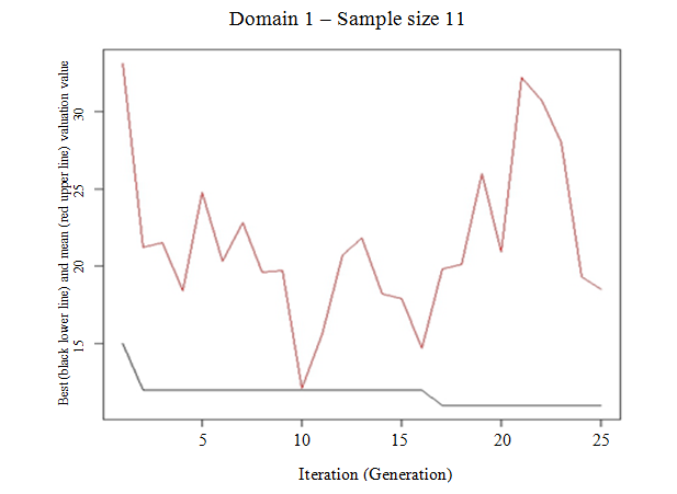
The graph in figure 4.2, obtained during the execution of the program, shows the convergence of the algorithm. In the graph, two different curves are reported: the lower one is related to the best solution found until the $k^{th}$ iteration (as the best solution is memorised, it can only decrease as the algorithm proceeds); the upper one reports the mean of the 10 solutions evaluated in each iteration.

Figure 4.2 Best and mean evaluation values during GA execution

Description for figure 4.2

Figure 4.2 Best and mean evaluation values during GA execution

The resulting best solution is $v = (4, 1, 3, 4, 1, 3, 3, 2) .$ It corresponds to the stratification reported in table 4.3, with an allocation vector $a = (3, 2, 4, 2) .$

Table 4.3
Information concerning final strata Table summary
This table displays information concerning final strata. The information is grouped by Aggregated stratum, Original atomic strata, ( X ₁, X ₂), N, Y ₁, Y ₂ (appearing as column headers).
Aggregated stratum	Original atomic strata	( X ₁, X ₂)	N	Y ₁		Y ₂
Aggregated stratum	Original atomic strata	( X ₁, X ₂)	N	Mean	Standard deviation	Mean	Standard deviation
1	2,5	(1,2) or (2,2)	41	4.16	0.45	1.30	0.19
2	8	(3,3)	26	5.88	0.49	2.10	0.22
3	3,6,7	(1,3) or (2,3) or (3,2)	33	5.06	0.38	1.80	0.33
4	1,4	(1,1) or (2,1)	50	1.46	0.17	0.25	0.10

In conclusion, by applying the genetic algorithm, we succeeded in finding the optimal solution by exploring only $25 \times 10 = 250$ alternative stratifications instead of the 4,140 belonging to the universe of partitions.

In order to verify that this result is not due to a "lucky strike�, we perform different executions of the algorithm: each execution iterates 10 times the application of the genetic algorithm, varying the values of the parameter "number of iterations�. Results are reported in table 4.4.

Table 4.4
Capability of GA to find the optimal solution
Table summary
This table displays the capability of GA to find the optimal solution. The information is grouped by Execution of the GA (10 times each), Value of parameter "number of iterations� in the GA, Solutions with n = 11 (optimal), Solutions with n = 12, Solutions with n = 14 (appearing as column headers).
Execution of the GA (10 times each)	Value of parameter "number of iterations� in the GA	Solutions with n = 11 (optimal)	Solutions with n = 12	Solutions with n = 14
(a)	25	5	4	1
(b)	50	7	3	-
(c)	100	9	1	-
(d)	200	10	-	-

In execution (a), we discover that, with only 25 iterations, to succeed in finding the optimal solution is actually a "lucky strike�, as in half of the trials the found solution is higher than the optimal. But increasing the number of the iterations up to 200 (execution (d)), the genetic algorithm proves to be reliable with respect to its capability to reach optimality, as in all the trials the optimal solution is found.

As for the number of the strata corresponding to the found optimal solutions, on average it is 4, with a range of $[3, 5] .$

Finally, we also want to verify that the found solutions are compliant with the precision constraints (maximum CV equal to 5% for both target variables). So, in execution (d) (iterations $= 200$ ), for each one of the 10 produced solutions we proceed to draw 1,000 samples from the frame and to calculate the related CV's. Corresponding results are shown in figure 4.3: the average of CV's for the first target variable (Petal.Lenght) is around 3%, while for the second one is around 5%. So, we can say that, on average, precision constraints have not been violated.