5 Discussion

Jan de Haan and Rens Hendriks

Previous | Next

5.1  Comparing GREG to SPAR

The most interesting question arising from Section 4 is: why are the GREG and SPAR index numbers so similar in spite of their very different construction methods? It is not remarkable that the trends are similar: although the GREG index does not rely on the matched-model methodology, this index does aim at the same target as the SPAR index. If the sample sizes $n^0$ and $n^t$ would approach the population size $N^0$ $–$ which in reality will of course never happen $–$ then both price indexes approach the value change of the fixed housing stock. Put differently, the two methods are both asymptotically unbiased or 'consistent'.

What may come as a surprise is that the GREG index exhibits roughly the same amount of volatility over time as the SPAR index. To understand the reason why, recall that, with OLS, the regression residuals sum to zero in every time period. This implies ${\displaystyle {\sum }_{n\in S^0}{p}_n^0}/n^0={\displaystyle {\sum }_{n\in S^0}{\widehat{p}}_n^0}/n^0$ and ${\displaystyle {\sum }_{n\in S^t}{p}_n^t}/n^t={\displaystyle {\sum }_{n\in S^t}{\widehat{p}}_n^t}/n^t.$ For the basic regression models (3.1) and (3.5), the SPAR index can thus alternatively be written as

$${\widehat{P}}_{\text{SPAR}}^{0t}=\frac{{\displaystyle \sum _{n\in S^t}{\widehat{p}}_n^t}/n^t}{{\displaystyle \sum _{n\in S^0}{\widehat{p}}_n^0}/n^0}\left[\frac{{\displaystyle \sum _{n\in S^0}{a}_n^0}/n^0}{{\displaystyle \sum _{n\in S^t}{a}_n^0}/n^t}\right]=\frac{({\widehat{\alpha }}^t+{\widehat{\beta }}^t{\overline{a}}^{0(t)})/{\overline{a}}^{0(t)}}{({\widehat{\alpha }}^0+{\widehat{\beta }}^0{\overline{a}}^{0(0)})/{\overline{a}}^{0(0)}}=\frac{{\widehat{\alpha }}^t/{\overline{a}}^{0(t)}+{\widehat{\beta }}^t}{{\widehat{\alpha }}^0/{\overline{a}}^{0(0)}+{\widehat{\beta }}^0},\left(5.1\right)$$

using (3.2) and (3.6) for $n\in S^0$ and $n\in S^t,$ respectively, where ${\overline{a}}^{0(0)}={\displaystyle {\sum }_{n\in S^0}{a}_n^0}/n^0$ and ${\overline{a}}^{0(t)}={\displaystyle {\sum }_{n\in S^t}{a}_n^0}/n^t$ for short. There is a striking similarity between the last expression on the right-hand sides of (5.1) and (3.10). The only difference is that the SPAR index (5.1) divides the coefficients ${\widehat{\alpha }}^0$ and ${\widehat{\alpha }}^t$ by the sample means of appraisals, ${\overline{a}}^{0(0)}$ and ${\overline{a}}^{0(t)},$ whereas the GREG index (3.10) divides them both by the fixed, non-stochastic population mean ${\overline{a}}^0.$ Essentially, the SPAR index is a fully sample-based estimator of the GREG index.

Compared with the SPAR method, the GREG approach eliminates one source of sampling error, i.e., the sampling variability of the mean appraisals. In accordance with generalized regression theory, we would intuitively expect the GREG method to reduce the sampling error of the price index and produce a less volatile time series (under the reasonable assumption that ${\overline{a}}^{0(t)}$ and ${\widehat{\alpha }}^t$ are uncorrelated across periods $t=0,\dots ,T).$ Put differently, while the GREG method has been designed as an improvement over the ratio of sample means, we might have expected it to work as a smoothing procedure for the SPAR index also. But, as was shown in Section 4, in practice this is hardly the case. This result can be explained as follows.

The variance reduction of the GREG index relative to the SPAR depends on the value of the intercept terms from the regressions in periods 0 and $t.$ If the regression lines passed exactly through the origin $({\widehat{\alpha }}^t={\widehat{\alpha }}^0=0),$ then the GREG index and SPAR index would both be equal to the ratio of the slope coefficients ${\widehat{\beta }}^t/{\widehat{\beta }}^0$ and no reduction in variance would be achieved. In the less extreme case, when ${\widehat{\alpha }}^t$ and ${\widehat{\alpha }}^0$ are close to 0 and the ratios ${\widehat{\alpha }}^t/{\overline{a}}^0,{\widehat{\alpha }}^t/{\overline{a}}^{0(t)},{\widehat{\alpha }}^0/{\overline{a}}^0$ and ${\widehat{\alpha }}^0/{\overline{a}}^{0(0)}$ in (3.10) and (5.2) are very small compared to ${\widehat{\beta }}^t$ and ${\widehat{\beta }}^0,$ the GREG and SPAR indexes will differ only slightly and the variance reduction will be marginal; see also the Appendix.

The latter is indeed what happens in practice, as can be seen from Figures 5.1 and 5.2 where the values of ${\widehat{\alpha }}^t/{\overline{a}}^0$ and ${\widehat{\alpha }}^t/{\overline{a}}^{0(t)}$ and those of ${\widehat{\beta }}^t$ are plotted over time. The ratios ${\widehat{\alpha }}^t/{\overline{a}}^0$ and ${\widehat{\alpha }}^t/{\overline{a}}^{0(t)}$ are remarkably similar and small as compared to the ${\widehat{\beta }}^t’\text{s}\text{.}$ Although we cannot ignore those ratios, it is the change in ${\widehat{\beta }}^t$ that mainly drives the GREG and SPAR indexes. The SPAR index is not only a fully sample-based estimator of the GREG index, as mentioned above, it appears to be almost as efficient.

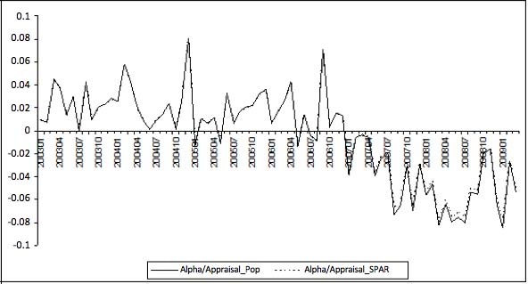
Description for figure 5.1

Figure 5.1  Intercepts divided by appraisal means

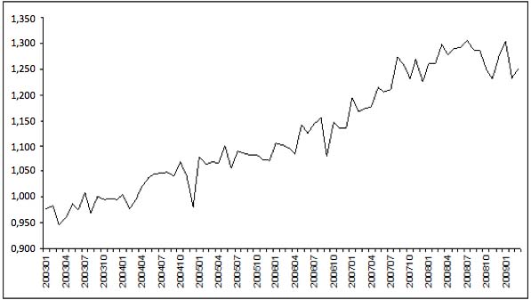
Description for figure 5.2

Figure 5.2  Slope coefficients

5.2  The volatility of the slope coefficient

Several factors may have contributed to the volatility of the slope coefficients ${\widehat{\beta }}^t$ in our regressions of selling prices on appraisals and hence of the GREG and SPAR indexes. We will briefly discuss three of these factors: sample mix change, heteroskedasticity and outliers.

A sample of houses can be viewed as a sample of locations, or addresses, since houses are attached to the land they are built on. A change in the sample mix is nothing else than a change in the observed mix of locations at the lowest level. A location mix change affects the sample composition in terms of the average quality characteristics of the properties, such as the number of rooms, surface area, etc. In our simple framework, where we observe only one (non-physical) characteristic, namely the appraised value, a location mix change boils down to a change in the sample distribution of the appraisals. This, together with any varying price changes across market segments, induces a change in the sample distribution of the ratios $p_n^t/a_n^0,$ which in turn leads to a change in ${\widehat{\beta }}^t$ in the two-variable regression model (3.5).

Other than by stratification there is little we can do about the effect of changes in the sample mix of locations (but stratifying by province and type of dwelling did not help much), so the volatility of ${\widehat{\beta }}^t$  and therefore of the GREG and SPAR indexes, will be difficult to reduce. Controlling for location at the address level is also impossible in hedonic imputation methods. Here, the effect of (location) mix change is mitigated by controlling for region plus a range of physical characteristics. However, this does not necessarily mean that hedonic imputation will produce more stable index series than the GREG or SPAR methods. Most standard hedonic models fit the cross sectional data less well than our model does, and the characteristics' coefficients typically exhibit a great deal of variability over time. So maybe it is not surprising that Bourassa, et al. (2006) find that "the SPAR index [….] reliably tracks house price changes, but exhibits less volatility than index methods that require more parameter estimates.�

We can alternatively look at the variability of the slope coefficient from a purely statistical perspective. It is well known that in a two-variable model the OLS estimator ${\widehat{\beta }}^t$ can be written as

$${\widehat{\beta }}^t=r(p^t,a^0)\frac{s(p^t)}{s(a^0)},\left(5.2\right)$$

where $r(p^t,a^0)$ denotes the sample correlation coefficient in period $t$ between selling prices and appraisals, which is equal to the square root of $R^2;s(p^t)$ and $s(a^0)$ are the corresponding sample standard deviations. A comparison of Figures 4.1 and 5.2 suggests that sudden changes in $R^2$ are largely responsible for the volatility of ${\widehat{\beta }}^t.$ In December 2004 for example, a substantial drop in $R^2$ coincides with a significant decrease of ${\widehat{\beta }}^t$ (and with a decrease in the GREG and SPAR indexes, as shown by Figure 4.4).

Least squares regression can either be weighted or unweighted. In the absence of heteroskedasticity, i.e., when the variance of the errors is constant, OLS should be used. Weighted Least Squares (WLS) is preferred if there is evidence of heteroskedasticity; using appropriate weights, WLS will lead to more stable coefficients than OLS. In this case the unweighted sample sum of the residuals differs from zero so the estimator (3.9) has to be applied. To facilitate the interpretation of the GREG index and the comparison with the SPAR index, in Section 3 we assumed away the problem of heteroskedasticity and restricted ourselves to OLS. Note that the (OLS) GREG estimator (3.10) remains asymptotically design unbiased if heteroskedasticity is present.

The most interesting form of (classical) heteroskedasticity $–$ and, given our data set, the only form we would have been able to reduce $–$ would arise if the variance of the errors of our regression model (3.5) depended on the appraisal value, being the only regressor. However, the residuals from our OLS regressions do not point to substantial heteroskedasticity of this type. This is illustrated in Figure 5.3 for three months, including the base period (January 2003), where the sale prices are plotted against the appraisals; the regression lines are also given. To be sure, we also performed the White (1980) test. This test did not point towards the presence of this form of heteroskedasticity either.

 

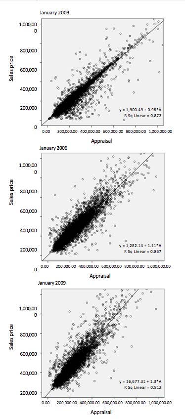
Description for figure 5.3

Figure 5.3  Scatter plots and regression lines

Our initial data set of sale prices and appraisals included some obvious outliers. To estimate the GREG index we therefore made use of a cleaned data set that has been prepared to compute the official Dutch house price index. Statistics Netherlands applies several data cleaning procedures. Houses that were sold more than once in a month are excluded from the data set. To delete entry errors and outliers that may unduly affect the results, properties with sale prices or appraisals below $€$10,000 or above $€$5,000,000 and properties with 'unrealistic' sale price-appraisal ratios are also removed. The removal of 'unrealistic' observations is done by looking at the distribution of the logarithm of the sale price-appraisal ratios; all observations are deleted for which the log ratio differs more than 5 standard deviations from the mean. For more information, see Statistics Netherlands (2008).

These procedures are rather arbitrary. For regression-based estimators such as the GREG it is more appropriate to delete observations with high leverage, i.e., to delete those sample units that have a big impact on the regression coefficients when they are excluded from the sample. A well-known measure in this context is the DFBETA of a sample unit (Cook and Weisberg 1982). Since the SPAR can be written as a regression-based index, this measure could be used here as well to detect and delete outliers. The scatter plots in Figure 5.3 show that the cleaned data set still contains some big outliers. Whether these have high leverage, and whether removing them will reduce the volatility of the ${\widehat{\beta }}^t’\text{s}$ and the GREG and SPAR indexes, remains to be seen.

5.3  Some further points

The GREG method is based on the premise of a fixed housing stock. That is, we have assumed that there are no entries (e.g., newly-built houses) or exits (discarded houses) and that housing quality remains fixed over time. Our approach is non-symmetric in that we condition on the base period stock. From an index number point of view we estimate a Laspeyres price index for the housing stock where the quantities are all equal to 1 because every house is treated as a unique property. An equally justifiable approach would be to measure the price change of the current period stock, which includes additions to the stock in each period, using a Paasche index. Taking the geometric mean of both indexes would lead to the Fisher index. The Fisher index is a preferred measure of price change due to its symmetric form. The construction of a Fisher-type GREG index is, however, infeasible since the Paasche component requires real time assessed values for houses that are new to the stock, which are obviously not available.

The assumption of a fixed (base period) housing stock can be relaxed through annual chaining, provided that the housing stock is re-assessed annually. This is the current state of affairs in the Netherlands; in the past, assessments were undertaken once every three or four years. Annual updating of the appraisals might also adjust for quality changes of the properties, to some extent at least, because the updated appraisals likely account for major repairs, remodelling and depreciation.

One final remark is in order. For some purposes it is desirable to decompose the overall house price index into two components: a component that measures the change in the price of the structure and a component that measures the change in the price of the land. Neither our GREG method nor SPAR and repeat sales methods are fit for that purpose. Hedonic imputation methods might work, notwithstanding practical problems like multicollinearity; see Diewert, de Haan and Hendriks (2012) for a first attempt. If data on structure size, plot size and other price-determining attributes became available for all properties in the housing stock, then we would be able to estimate a "hedonic imputation GREG index�, including the land-structure split. The chances of getting such data in the Netherlands are unfortunately negligible.

Previous | Next