How Much Thicker is the Canada–U.S. Border? The Cost of Crossing the Border by Truck in the Pre- and Post 9/11 Eras

View the most recent version.

Archived Content

Information identified as archived is provided for reference, research or recordkeeping purposes. It is not subject to the Government of Canada Web Standards and has not been altered or updated since it was archived. Please "contact us" to request a format other than those available.

Archived

This page has been archived on the Web.

by W. Mark Brown

Skip to text

• Abstract
• Executive summary
• 1 Introduction
• 2 Data development
  • 2.1 Trucking Commodity Origin and Destination Survey
  • 2.2 Trucking price index
  • 2.3 Data description
• 3 Econometric model
  • 3.1 Specification
  • 3.2 Model set-up
  • 3.3 Results
• 4 Ad valorem trucking costs
  • 4.1 Calculation of ad valorem costs
  • 4.2 Ad valorem transportation cost tariff equivalents
• 5 Conclusion
• Appendix

Text begins

Abstract

In the aftermath of 9/11, a new security regime was imposed on Canada–U.S. truck-borne trade, raising the question of whether the border has ‘thickened.’ Did the cost of moving goods across the border by truck rise and, if so, by how much, and have these additional costs persisted through time? Building on previous work that measured the premium paid by shippers to move goods across the Canada–U.S. border by truck, from the mid- to late 2000s, this paper extends the time series back to 1994, encompassing the pre- and post-9/11 eras. The analysis shows that the premium paid to move goods across the border rose, from 0.3% of the value of goods shipped prior to 9/11, to about 0.6% after 9/11, with these higher costs persisting through to the late 2000s. Whether these additional costs are imposed on the export or import leg of the cross-border journey depends on the balance of cross-border trips, with the export leg bearing these costs until about 2005, and increasingly the import leg thereafter.

Keywords: border costs, international trade, transportation costs.

Executive summary

Building on previous work that focused on the mid- to late 2000s (Anderson and Brown 2012; Brown and Anderson 2015), this paper extends the period of analysis back to 1994. This much longer period was marked by substantial changes in the Canada–U.S. trading relationship. It encompasses the terrorist attacks on 9/11 that ushered in a new and evolving security regime and a switch in the balance of Canada–U.S. truck-borne trade. These changes had potentially two countervailing effects on the rates charged to transport goods to the United States by truck. Following 9/11, increased delays at the border and additional border regulations may have increased the costs borne by trucking firms when shipping goods to the United States, putting upward pressure on prices. However, in the ensuing years, falling relative demand for the U.S.-bound leg of the cross-border round trip put downward pressure on prices.

Statistics Canada’s Trucking Commodity Origin and Destination Survey is used to assess the degree to which it costs more to cross the border in the pre- and post-9/11 eras. On a shipment basis, it measures the revenue of trucking firms and, by implication, the cost borne by shippers for both domestic and cross-border shipments. By comparing these, it is possible to measure whether trucking firms charge a higher price to ship goods to and from the United States and to assess whether those prices have changed over time.

The paper finds the following:

• At the micro level, there is evidence that border compliance costs are reflected in prices. After 2001, fixed costs per shipment rose more rapidly on exports. Much of this rise occurred in 2004, coinciding with the implementation of new border regulations imposed by the United States. There is less evidence that prices rose in reaction to delays at the border in the immediate aftermath of 9/11.
• From 2004 onward, line-haul costs (costs that vary with distance) on exports rose at a slower pace than those on imports and domestic trade, and this occurred at a time of declining demand for the export leg and increasing demand for the import leg of the cross-border trip.
• Between 1994 and 2000, it cost on average 16.3% more to ship goods across the border than to ship the same goods the same distance domestically. The premium on cross-border shipments remained at about the same level until 2000, after which it rose to 25.1% in 2005 and remained relatively high thereafter.
• The leg of the journey that bears these extra costs switched between 2005 and 2009, reflecting changing relative demand for the export and import legs. In 2005, the premium on the export leg was 30.0%, while the premium on the import leg was 20.3%. By 2009, the premium on the export leg had fallen to 17.1% and risen on the import leg to 25.6%.
• The ad valorem tariff equivalent of the premium on cross-border trade over the 1994 to 2000 period averaged 0.33%, but almost doubled to 0.62% between 2005 and 2009. While the tariff equivalent is relatively small, its effect will be magnified for goods such as auto parts that pass over the border several times as they move through the various stages of the production process.

The costs measured here are only part of the total cost of shipping goods across the border. The institutional costs borne directly by exporting firms for matters like customs administration have been estimated to be as great as or greater than the costs passed on to them by freight carriers (Taylor, Robideaux and Jackson 2004). Furthermore, increased variability in border-crossing times may cause shippers to maintain buffer inventories on the other side of the border, which would not be reflected in carrier revenues (Anderson and Coates 2010).

1 Introduction

After 9/11, a new security regime was imposed on the movement of goods across the Canada–U.S. border, which led many to ask whether the border has ‘thickened.’ That is, did the cost of moving goods across the border rise, and, if so, by how much? The purpose of this paper is to assess the additional cost of moving goods across the border by truck in the post-9/11 era, compared with the pre-9/11 era. Trucks are the primary mode by which goods cross the border, transporting half of the dollar value of exports to the United States and just over two-thirds of imports.^{Note 1} This paper builds on previous work that measured the premium paid by shippers to move goods across the Canada–U.S. border by truck, from the mid- to late 2000s, by extending the time series back to 1994, encompassing the pre- and post-9/11 periods (Anderson and Brown 2012; Brown and Anderson 2015).

The costs of crossing the border can be divided into three basic types: formal tariff barriers, non-tariff barriers, and the cost of the transport system itself. The latter is the focus of this paper—in particular, the border-related costs incurred by trucking firms that are passed on to their customers through higher prices.^{Note 2} These costs may stem from increased wait times or their changeability, and from the cost of complying with additional border regulations often aimed at speeding passage across the border (e.g., implementation of a series of security protocols required for participation in trusted-trader programs).

To date, considerable work has been undertaken to examine whether the post-9/11 security regime has had a detrimental effect on Canada–U.S. trade (see Globerman and Storer [2008, 2009], Grady [2008], and Burt [2009]). These studies assess the impact of the new security regime by observing the volume of trade prior to and after 9/11 using standard gravity-style trade models. An unaccounted for drop in the volume of trade is seen as evidence that border thickening resulted in higher delivered prices and a concomitant drop in the quantity of exports demanded in the United States. The evidence from these models is mixed, with Globerman and Storer (2008; 2009) and Grady (2008) finding evidence of a drop in the volume of trade, while Burt (2009) finds little evidence of this effect.

While the costs borne by carriers in the wake of 9/11 may be reflected in prices, so too will other factors that influence the Canada–U.S. trading relationship in the 2000s. One of the most important factors is the balance of Canada–U.S. truck-borne trade, which determines which leg of the cross-border round trip constitutes the ‘backhaul.’ Carriers, when they take a contract,

• “…must commit to the maximum transport capacity required for a round-trip and, therefore, face a logistics problem: there is an opportunity cost associated with returning empty (‘backhaul problem’), and that opportunity cost depends on the shipping direction.” (Behrens and Picard 2011, 281)

The backhaul problem is well known (see Felton [1981] and Jonkeren et al. [2011]). If the truck is empty on the return trip, the opportunity cost of that leg is zero (Behrens and Picard 2011). Hence, the carrier will have an incentive to undercut other carriers on that leg, putting downward pressure on prices. Of course, the opposite occurs for the leg with a high level of demand. Prices on the leg with low demand (the ‘backhaul’) and on the leg with high demand (the ‘fronthaul’) can differ greatly. For instance, reflecting the large imbalance in U.S.–China trade, in 2005, it cost $1,400 to ship a container from China to the United States, but only $400 to $500 for the return journey (Behrens and Picard 2011).

Through the study period, the relative demand for trucking goods to and from the United States has shifted. During the 1990s, the implementation of the Canada–United States Free Trade Agreement and the North American Free Trade Agreement brought about expanded trade with the United States, with a rising share of manufacturing output exported across the border (Baldwin and Yan 2012). With the balance of trade favouring Canada during this period, export trips were likely the fronthaul and import trips the backhaul. In the 2000s “…the worldwide resource boom…led to higher prices for Canadian commodity exports, an increase in the Canada–U.S. exchange rate, [and] a decline in the competitiveness of the Canadian manufacturing sector in U.S. markets” (Baldwin and Yan 2012, 7). For a cross-border round trip, the fronthaul may have switched from the journey to the United States to the journey home. The obvious implication is that during a period when there should be upward pressure on the price of shipping goods to the United States, because of the new security regime, there was also downward pressure on prices because of changes in the relative demand for the two legs of the U.S. round trip.

Disentangling these effects cannot be accomplished through aggregate trucking price indices, because they reflect the net of these countervailing effects through the 2000s. Required is an econometric analysis of the prices charged by motor carriers at the micro level, which permits the breakdown of the effect of fixed and variable (line-haul) costs on these prices. Assuming that border compliance costs are reflected in the fixed cost of cross-border movements and that changes to the fronthaul/backhaul’ portions of the journey are reflected in line-haul costs, these two effects can be identified separately.

Statistics Canada’s Trucking Commodity Origin and Destination (TCOD) Survey is used to assess the impact of these effects. It samples waybills of for-hire trucking firms to measure the characteristics of their shipments (for example, revenue, weight, distance shipped and commodity type) for domestic and cross-border shipments, primarily to the United States. The TCOD Survey provides a means to measure trucking costs—that is, the cost to shippers of moving their goods between origin and destination.

This paper uses a dataset that, while having much in common with the one used by Anderson and Brown (2012), is qualitatively different in several fundamental respects. First, and most obvious, the dataset was extended back to 1994. This was not a trivial task, because the wholesale redesign of the TCOD Survey between 2003 and 2004 meant considerable care had to be taken to ensure the consistency of the time series over the period and the robustness of the econometric estimates to changes to the survey design. Second, since the TCOD Survey does not measure the value of goods shipped, they had to be estimated by multiplying the tonnage shipped by the value per tonne on a commodity basis. Anderson and Brown (2012) did this by using a relatively aggregate set of commodities. Since then, a set of much more fine-grained commodity value per tonne estimates became available for imports and exports, providing an opportunity to improve the accuracy of the estimated value of goods shipped. Third, commodity import and export price indices were used to estimate the nominal value per tonne over the period. Once again, these are based on a more fine-grained set of commodities than that used in previous work. Finally, the database was rebuilt on a quarterly rather than an annual basis. This was necessary because many of the key events over the period that might affect the price of goods shipped across the border needed to be measured using a quarterly rather than an annual time scale. For instance, addressing the effect of delays at the border immediately after 9/11 required quarterly data, because these delays dissipated relatively quickly after the event. Because of these changes to the methods, the discussion takes care to outline their implementation.

The next section describes the methods used to develop a comprehensive measure of trucking costs. This entails a more detailed description of the TCOD Survey dataset and the steps taken to ensure the comparability of these survey data through the study period. Section 3 presents a multivariate analysis that takes into account potential differences between cross-border and domestic shipments to arrive at an estimate of their relative costs. This is followed by the presentation of ad valorem estimates of trucking costs (Section 4) and, in particular, the ad valorem tariff equivalent of shipping goods across the border, which is used to measure the degree and persistence of border thickening. The last section provides a brief conclusion, summarizes the results of the analysis and outlines some caveats in interpreting the data.

2 Data development

2.1 Trucking Commodity Origin and Destination Survey

The Trucking Commodity Origin and Destination (TCOD) Survey measures (1) the output of the for-hire trucking sector and (2) the volume of commodities moved by truck (Gagnon and Trépanier n.d.). As noted above, the survey measures on a shipment basis the tonnes shipped, the distance shipped, the origin and the destination, and the revenue earned by the carrier. The revenue earned by the carrier from each shipment reported by the TCOD Survey is used here to assess the relative costs of domestic and cross-border transportation. The question arises as to whether the revenue from a specific shipment is a good proxy for the total cost of transportation. This might not be true if carriers do not pass the full cost of crossing the border onto shippers. However, this would imply that carriers accept lower profit margins for cross-border shipments than for domestic shipments, which seems unlikely.

The survey underwent a major revision in 2004. In concrete terms, the TCOD Survey methodology changed in three ways (see Gagnon and Trépanier [n.d].). First, its sampling routine changed from two stages to four stages, and this affects the weights used on the file. In unpublished work undertaken by Transport Canada, the four-stage weights were substituted for two-stage weights in 2001 and 2002. This substitution had little effect on the prices.

Second, the scope of the survey changed in 2004. This involved the inclusion of short-distance carriers (North American Industry Classification System [NAICS] 48411 and 48422) and used household and office goods moving (NAICS 48421). Shipments of 25 kilometres or less were also now included in the sample.

Finally, data processing and estimation were changed. These seemingly small changes can have a profound effect when comparing microdata-based estimates over time. For instance, less micro-editing is done on the modern file, increasing the level of errors in the file and potentially leading to errors in variable-driven bias. As will become apparent below, this change in methodology necessitates a careful treatment of the data.

2.2 Trucking price index

Given the changes in the survey methodology between 2003 and 2004, at issue is whether the two series are comparable. To assess whether there are significant breaks in the series between 2003 and 2004, a non-parametric trucking price index is developed (see Brown and Zhu [2012]). The development of the price index serves two additional purposes. First, it can be seen as an initial step in determining whether there has been a rise in truck prices on cross‑border movements after 2001. Second, it provides a means to identify trends in prices that should be taken into account in the econometric modelling.

The cost of moving goods by truck depends on the origin and destination, the distance, the weight, and the type of shipment. To account for these factors, the price per tonne‑kilometre is calculated by cross-classifying shipments across these classes:

$$P_k^y=\frac{r_k^y}{{\left(td\right)}_k^y},(1)$$

where $P_k^y$ is the price for the $k^{th}$ class in year $y$, $r_k^y$ is the revenue,^{Note 3} and tonnes $(t)$ multiplied by distance $(d)$, $td$, is the number of tonne-kilometres. The $k^{th}$ class is defined by 18 origin–destination (domestic and cross-border) pairs, four distance classes, three weight classes, and 40 commodity classes, resulting in a maximum of about 8,640 classes.

The next step is to develop a price index that aggregates across these classes of shipments to provide an aggregate measure of price changes over time. In this instance, the price index might be more accurately referred to as a unit value index, because the nature of the service is permitted to change through time. Nevertheless, the ‘price index’ terminology is kept in order to maintain consistency with the literature.

To capture aggregate price changes, a Törnqvist price index, $C\left(p^y\right)$, is calculated by aggregating the logs of the price change for all classes $k$, weighted by the average of the revenue share for each class for two consecutive years :

$$C\left(p^{y+1}\right)=c\left(p^y\right)\times \exp \frac{1}{2}{\displaystyle {\sum }_k\left\{\left[\ln \left(P_k^{y+1}\right)-\ln \left(P_k^y\right)\right]\times \left[\ln \left(S_k^{y+1}\right)-\ln \left(S_k^y\right)\right]\right\},} (2)$$

where $S_k^y$ is the revenue share for the $k^{th}$ class in year $y$, given by

$$S_k^y=\frac{r_k^y}{{\displaystyle {\sum }_k{r}_k^y}}. (3)$$

The price index is calculated for domestic trade and cross-border movements, divided into exports and imports. Chart 1 presents the price index after excluding short-distance carriers (NAICS 48411 and 48422) and movers (NAICS 48421). Also excluded are trips of 25 kilometres or less. While there is no serious break in the series between 2003 and 2004, there is a noticeable upward movement in domestic and import prices, and a less noticeable upward movement in export prices. Furthermore, the overall rise in prices after 2003 was stronger than expected based on the alternative prices series (see Brown and Zhu [2012]). Therefore, an additional step was taken to filter the data based on quality to ensure that relative price changes across trade types are not an artifact of changes to the survey methodology.

Description for chart 1

Quality is defined as a change in price between years for a given cell $k$ that is beyond some threshold value. The first step in developing this threshold value is to calculate the standard deviation, ${\sigma }^y$, of the average price change over all cells for year $y$. In turn, for each cell, the relative price change that corresponds to the number of standard deviations away from the mean is calculated:

$$n_k^y=\frac{\frac{{\overline{p}}_k^{y+1}-{\overline{p}}_k^y}{{\overline{p}}_k^y}}{{\sigma }^y},(4)$$

where $n_k^y$ is the number of standard deviations away from the mean for cell $k$ in year $y$. Key to the procedure is the identification of a year to measure the relative change in prices. The year 1998 is chosen because prices were relatively stable across the alternative price indices. For that year, the $\pm$25%^{Note 4} relative average price change corresponds to the following standard deviations away from the mean:

$$n_{k,0.25}^{1998}=\pm \frac{0.25}{{\sigma }^{1998}}. (5)$$

$n_{k,0.25}^{1998}$ is applied to all the other years. Hence, if $n_k^y$ is greater than $\left|n_{k,0.25}^{1998}\right|$, then that cell is excluded. Since this involves truncating both large increases and decreases in prices relative to the mean change in prices for each year, no upward or downward bias should be introduced. In addition to controlling for quality, the series are spliced between 2003 and 2004 using an alternative price series from the national accounts (see Brown and Zhu [2012]).

When these exclusions are applied and the series are spliced, the price indices for domestic trade and exports and imports undergo a significant shift (see Chart 2). First, domestic prices rise at a much slower pace in the post-2004 period, rising to a peak index value of 125, compared with 160 without the quality adjustment (see Chart 1). Export prices also rise at a slower pace after 2003, but import prices rise more rapidly. This is consistent with econometric estimates that suggest prices rose more rapidly for imports after 2003 than for exports (Anderson and Brown 2012), and with aggregate trucking price indices produced by the national accounts (Brown and Zhu 2012). This price pattern coincides with a shift in the trade regime, where truck‑borne imports by value and number of trips now outweigh exports (see Chart 3). That is, the backhaul portion of the round trip has switched from the import portion of the journey (from the Canadian perspective) to the export portion of the journey. In the econometric analysis, these exclusions for quality will be used as a robustness check.

Description for chart 2

Beyond the question of data quality, the substantive point to be taken from Chart 2 is that there is no discernible increase in trucking prices for exports after 2001, which would have been anticipated if carriers had incurred delays at the border and other border compliance costs and passed them on to shippers in the form of higher prices. Still, establishing whether this is truly the case requires more analysis, because of the countervailing effects of changes to the security regime and of shifting relative demand for export and import trips on prices. Distinguishing between these effects requires an econometric analysis at the micro level.

2.3 Data description

The primary purpose of this study is to measure the cost of shipping goods across the border. Before presenting estimates of these costs, several aspects of the aggregate data are examined, including the scope of the TCOD Survey, the types of carriers covered, and the trends in truck‑borne trade over the study period.

The TCOD Survey is limited to for-hire trucking firms based in Canada, and, therefore, it excludes foreign-based trucking firms operating in Canada and non-trucking firms with their own fleets (own-account trucking).^{Note 5} However, as Anderson and Brown (2012) note, the trucking costs derived from the TCOD Survey should be representative of the entire trucking sector because it accounts for the vast majority of the tonnage moved across the Canada–U.S. border. Furthermore, because the trucking sector is highly competitive^{Note 6} excess profits should be rapidly competed away, equalizing rates across in-scope and out-of-scope firms.

Using the industrial classifications, trucking firms (or carriers) are classified into three types: truckload, less-than-truckload and specialized. Truckload carriers specialize in moving loads between their origin and final destination, while less-than-truckload carriers specialize in moving multiple consignments between terminals where loads are consolidated at one end and broken down at the other. Specialized carriers are distinguished by the type of equipment used (e.g., tank trucks to move liquids). Each type represents a different trucking technology (truckload and less-than-truckload compared with specialized) and business model (truckload and specialized compared with less-than-truckload).^{Note 7} Owing to these differences, the various types of carriers may incur differing fixed and/or line-haul costs. For instance, specialized carriers are likely to have higher fixed costs and line-haul costs, because their capital costs are higher and they are less likely to obtain a backhaul, respectively. On the other hand, less-than-truckload carriers may incur higher fixed costs because of delays at the border caused by loads with multiple consignments.

Table 1 presents the basic characteristics of the sample. It reports the mean revenue, tonnage and distance per shipment for all carrier types. To ensure the estimates are more comparable between the 1994-to-2003 and 2004-to-2009 survey methodologies, the same sample and quality exclusions used in the development of the price index are applied. Perhaps as a result of these efforts, there is no apparent break in the time series for these shipment characteristics between 2003 and 2004, which is reassuring. The primary difference between cross-border shipments and domestic shipments is the distance travelled, which tends to be much less for domestic shipments. Hence, average revenues per shipment were higher for exports and imports than for domestic trade. Also, there has been a tendency for the distance shipped to increase for both exports and imports through the 2000s. As an aside, this pattern would be consistent with rising fixed costs, which tend to discourage short-distance shipments, for which fixed costs account for a larger portion of total costs.

3 Econometric model

3.1 Specification

This paper follows the basic pricing model developed by Brown and Anderson (2015). Presented here is a summary of that model. Trucking costs borne by carriers include a fixed component and a variable (line-haul) component. These can be incorporated into a simple pricing rule that takes into account both fixed costs $(\alpha )$ and variable (line-haul) costs per kilometre shipped $(\beta )$: $r_{ijl}=c_{ijl}=\alpha +\beta d_{ij}$, where $r$ is revenue (price charged) per shipment, $c$ is cost, $d$ is distance, and $i$, $j$, and $l$ index the origin, destination and shipment, respectively. This rule assumes that all economic profits are competed away, equating revenues and costs. Assuming further that firms set their price per kilometre on the basis of a full load (or average load) results in the following revenue function:

$$r_{ijl}=\alpha +\frac{\beta }{t^{\ast }}{d}_{ij}{t}^{\ast }, (6)$$

where $t*$ is the unknown tonnage (e.g., for a full load by weight) used for pricing purposes. Therefore, the implicit line-haul cost per tonne-kilometre using this pricing rule is $\beta /t^{\ast }$. This implies that for a load with a tonnage less than $t*$, the rate per tonne-kilometre would have to be scaled upward to ensure that the pricing rule, on a per-kilometre basis,^{Note 8} is maintained:

$$r_{ijl}=\alpha +\left[\frac{\beta }{t^{*}}+\varphi \left(t^{*}-t_l\right)\right]d_{ij}{t}_l=\alpha +\left(\frac{\beta }{t^{*}}+\varphi t^{*}\right)d_{ij}{t}_l-\varphi d_{ij}{t}_l^2,(7)$$

where $\varphi \left(t^{\ast }-t_l\right)$ is the scaling factor that is a linear approximation of the relationship between price per tonne-kilometre and the pricing rule per kilometre.

Equation (7) can be estimated using the following simple quadratic form:

$$r_{ijl}=\alpha +\delta d_{ij}{t}_l+\omega d_{ij}{t}_l^2, (8)$$

where $\delta =\beta /t^{\ast }+\varphi t^{\ast }$ and $\omega =-\varphi$, with the expectation that $\delta$ will be positive and $\omega$ negative.

Equation (8) is augmented by including an additional distance term to account for instances when there is no backhaul (deadheading), in which case the revenue per shipment is also a function of distance alone, reflecting the empty backhaul.^{Note 9} Therefore, the premium paid on the fronthaul is simply the rate $\gamma$ charged per kilometre for running empty multiplied by the distance and the probability $(P)$ of not obtaining a backhaul:

$$\gamma d_{ij}P=\nu d_{ij}.(9)$$

Finally, a squared distance term to account for any non-linear effect of distance on revenues, which may result if the probability of not obtaining a backhaul decreases with distance, and an error term are added to (8):

$$\begin{array}{l}{r}_{ijl}=\alpha +\delta d_{ij}{t}_l+\omega d_{ij}{t}_l^2+\nu d_{ij}+\phi d_{ij}^2+{\epsilon }_{ijl};\text{ or}\\ \text{ =}\underset{\text{fixed cost}}{\underbrace{\alpha }}+\underset{\text{line-haul cost}}{\underbrace{\left(\delta t_l+\omega t_l^2+\nu +\phi d_{ij}\right)d_{ij}}}+{\epsilon }_{ijl}. (10)\end{array}$$

3.2 Model set-up

To permit the effect of distance and tonnage on carrier revenues to vary across carrier types—truck-load, less-than-truck-load and specialized—separate models are estimated for each.^{Note 10} As with the price index, shipments of short-distance carriers and movers are excluded, as were shipments of 25 kilometres or less. Furthermore, the results are also presented with observations excluded from cells $k$ for which, in a given year, the change in price was large enough to call into question the quality of the data (see the price index discussion above).

The analysis uses a pooled set of cross-sections from 1994 to 2009. Over such a long period, fixed and variable costs are expected to change and as a result the base model is augmented in two ways. First, since diesel prices are a primary driver of variable costs, a diesel price index^{Note 11} is added to the model $(l_{dsl})$. The Trucking Commodity Origin and Destination (TCOD) Survey reports the date of shipment by quarter, and, therefore, a quarterly diesel price is used in the estimation.^{Note 12} Because prices often take time to adjust to changes in costs (see Blinder [1991]; Amirault, Kwan and Wilkinson [2006]; de Munnik and Xu [2007]), the diesel price index is lagged by two quarters. The diesel price index enters the model through its interaction with tonne-kilometres $(dt)$ and tonne-kilometres $\times$ tonne $(d{t}^2)$.

Second, additional controls for time need to be added to the model. There are two alternative approaches for including these time effects. The standard approach is to add time-fixed effects and interact these with the measures of variable costs. This leads to a larger number of (likely volatile) coefficients to interpret and does not address the core issue of how variable and fixed costs have changed as a result of specific events. The alternative approach is to add two time trends to the model: one for fixed costs and the other for variable costs. The trends enter the model in the form of a spline (piecewise regression) and measure the marginal quarterly change in the relevant coefficient value.

The disadvantage of time trends is that they necessitate the specification of turning points (knots), and this invites the possibility of data mining. The time trends themselves require justification. For fixed costs, the knots correspond to specific events. Based on survey evidence (Transport Canada 2005), the primary cost to carriers resulting from tightened border security following the events of 9/11 was increased delays at the border and inland. Inland delays stem from the requirement to notify the U.S. Customs and Border Protection (CBP) before a truck reaches the border.

These two sources of delays have different time signatures. The most acute delays at the border occurred during the immediate aftermath of the events of 9/11. These are taken into account by including three knots. The first is added between the second and third quarters of 2001, the second knot between the third and fourth quarters of 2001, and the third knot between the second and third quarters of 2002. These enable fixed costs to change during the quarter including 9/11 and during the three subsequent quarters; that is, the last quarter of 2001 and the first two quarters of 2002.

The second source of delay occurs inland and, as noted above, stems from new regulations requiring the transmission of cargo manifests before trucks reach the border. These regulations were implemented well after the events of 9/11. On July 23, 2003, pursuant to the Trade Act of 2002, the CBP announced its intent to amend customs regulations to require prior notification before entry. This was followed by the publication of the final rules on December 5, 2003, and the announcement on August 17, 2004, of the date of compliance, which, for major ports of entry, was November 15, 2004.

The consequence of these changes is that carriers had to adjust or augment their logistics systems to transmit their manifests to customs brokers well ahead of time. As noted by Transport Canada (2005, 6), “this new requirement puts an end to the ‘load-and-go’ approach whereby drivers could simply load, pick up their paperwork and show up at the border unannounced.” Carriers have to transmit their manifests to the CBP at least an hour before reaching the border, unless they are certified in the Free and Secure Trade (FAST) program, in which case a 30-minute notice is sufficient. Note that, because the electronic manifests are transmitted through customs brokers, the time required is typically more than an hour—often two hours (Transport Canada 2005). Hence, shipments within two hours of the border may be delayed further, and, overall, carriers incur more coordination costs.

When carriers reacted to these new regulations is unknown. On one hand, the prices charged by carriers might not have changed until after the regulations were implemented, which was not until the middle of the last quarter of 2004. On the other hand, the publication of the final rules at the end of 2003 and the compliance date of August 2004 may have pushed carriers to implement a series of costly measures in the run-up to the implementation of the new regulations.

To understand why the publication of the rules may have increased carrier costs, note that carriers gain a competitive advantage if they are qualified for the FAST program. A prerequisite for qualification in FAST, however, is enrolment in the Customs-Trade Partnership Against Terrorism (C-TPAT). C-TPAT is intended to increase the security of the supply chain by having participating firms implement a set of security measures (e.g., installing security cameras, lighting and fencing [Transport Canada 2005]). In addition to enrolment in C-TPAT, membership in the FAST program requires that U.S. importers, motor carriers and drivers meet a set of security criteria. Carriers incur considerable upfront costs to qualify for these programs, and these costs would have been incurred before the implementation of the new regulations at the end of 2004. As a result, prices may have risen prior to the imposition of the new regulations. Therefore, to account for these new regulations, additional knots were added between the first quarter of 2004 and the second quarter of 2004, the last quarter of 2004 and the first quarter of 2005.

In 2004, there was a change in the survey methodology, in addition to important regulatory changes. To take into account the change in the survey methodology, knots were included for the first and second quarters of 2004.

Since the diesel price index allows line-haul (variable) costs to vary with time, the timeline for variable costs is simpler with only two knots. It attempts to take into account changes in the trade regime that might have switched the backhaul from the import portion to the export portion of the round trip to the United States. Hence, the marginal effect of the trend is permitted to change between 2003 and 2004, which corresponds to the point when the balance of truck-borne trade by value and trips shifts decidedly in favour of the United States (see Chart 3) and when the price indices for imports and exports diverge (see Chart 2). A second knot is included between the third and fourth quarters of 2008 to account for the effects of the global recession on prices. Other specifications of the line-haul trend were also tested. These included permitting the trend to vary for the economic slowdown of the early 2000s and for the change in survey methodology by allowing the influence of the trend to change during the first quarter of 2004. In both instances, the coefficients were insignificant and so the more parsimonious specification was chosen.

Description for chart 3

All variables in the model, including the time trend (and its interaction with tonne-kilometres), are further interacted with a column vector of trade-type binary variables $p$, where $p=\left(dxm\right)$ and $d$ is domestic trade, $x$ is exports, and $m$ is imports. This functional form allows for differing coefficients across trade types, which is essential for testing whether fixed costs, for instance, rose more rapidly for exports compared to domestic trade during the post-2001 period.

Finally, to account for variability in revenues across commodities, the model includes a vector of fixed effects, $\lambda$. Depending on the model, these include binary variables accounting for the commodity shipped at the five-digit level of the Standard Classification of Transported Goods, the carrier, or the carrier-commodity, where the commodity is measured at the two-digit level. Revenues may vary across commodities and/or carriers for many reasons. For instance, to ship higher-value commodities, carriers tend to charge more for a higher level of service in terms of speed and reliability.

Hence, in its final estimated form, the revenue equation is

$$\begin{array}{l}{r}_{ijl}=\alpha +x+m+\\ p\left[{\gamma }^p{q}^a+\left({\delta }^p{t}_l+{\delta }_{dsl}^p{I}_{dsl}{t}_l+{\delta }^p{q}^b{t}_l+{\sigma }^p{t}_l^2+{\sigma }_{dsl}^p{I}_{dsl}{t}_l^2+{\sigma }^p{q}^b{t}_l^2+{\nu }^p+{\nu }^p{q}^b+{\phi }^p{d}_{ij}+{\phi }^p{q}^b{d}_{ij}\right)d_{ij}\right]+ (12)\\ \lambda +{\epsilon }_{ijl},\end{array}$$

where $q^a$ and $q^b$ are column vectors corresponding to the fixed-cost and variable-cost trends and $\gamma$, $\delta$, $\sigma$, $\nu$, and $\phi$ are parameter row vectors that correspond to their respective trends. As a final econometric note, estimates of statistical significance are based on robust standard errors corrected for the correlation of errors across shipments transported by the same firm. It is important to cluster by carrier, because some carriers are sampled across years, and this may lead to correlated errors common to fixed-effect (panel-based) models (see Petersen [2009]). Correcting for the correlation of errors across shipments transported by the same firm addresses this problem (see Kézdi [2004]; Petersen [2009]).^{Note 13}

3.3 Results

By value, most of the truck-borne trade between Canada and the United States is carried by truckload carriers (Anderson and Brown 2012). Therefore, to simplify the exposition, the econometric estimates focus on truckload carriers (see Table 2), while the estimates for less-than-truckload carriers and specialized carriers are presented in the appendix.

There are two samples used in the analysis. The ‘full sample’ does not restrict the data set to take into account data quality, while the restricted sample eliminates observations of cells $k$ whose average revenues per shipment were deemed to have changed too much between years. There are no qualitative differences between the results of the full sample and the restricted sample (see Models 1 and 2).

Only after carrier-fixed effects are added do the results change qualitatively. When this is done, point estimates for the additional fixed costs associated with exports and imports fall, suggesting there are unobserved characteristics of carriers engaged in cross-border trade not accounted for in the model specification (e.g., carriers engaged in cross-border trade may provide a higher level of service and this is reflected in their fixed costs). As a consequence, the preferred model is Model 4, which controls for the carrier of the shipment and the commodity shipped, albeit at the two-digit level.^{Note 14} Model 5 has the same specification as Model 4 but uses the full sample. Its results are not qualitatively different than those of Model 4, and, therefore, it will be the basis for the analysis in the discussion to follow and for the predictions used in the next section.

As a point of departure for the discussion of the results, it is useful to relate the basic findings back to the model specified in Equation (10). First, fixed costs are always associated with shipments. Second, variable (line-haul) costs per kilometre increase with tonnes shipped, but this marginal effect decreases with the tonnage, which is consistent with at least a portion of firms setting prices on a per-kilometre basis. Costs generally increase with distance, and, when statistically significant, the effect of distance is typically non-linear, with its marginal effect decreasing with distance. The positive coefficient on distance may be interpreted as resulting from adding costs from the backhaul portion of the journey to the fronthaul in response to differences in the relative demand for the different portions of the round trip. These results hold regardless of the model specification and the type of trade.

At issue, of course, is how fixed and line-haul costs vary between domestic and cross-border shipments, and how these have changed over time. While Table 2 provides the coefficient estimates on time trends for fixed and line-haul-cost-related variables for domestic trade, exports and imports, discussing these coefficient estimates in detail would not provide the reader with an easily interpretable picture of how variable and fixed costs have varied over time. Instead, the discussion will focus on a set of figures that trace out the predicted fixed and variable costs across trade types over the 16-year study period. Only when necessary will reference be made to the econometric results reported in Table 2. The figures present predictions of fixed, line-haul, and fixed and line-haul costs based on the parameter estimates from Model 5 in Table 2.

For domestic shipments, the fixed costs per shipment was $103.60 ($101.20 constant + $2.40 trend) in the first quarter of 1994. Through the period from the first quarter of 1994 to the second quarter of 2001, fixed costs increased by a statistically significant $2.40 per quarter. The pace of change varied over the subsequent periods, but there was no significant change with the exception of the last three quarters of 2004.

Fixed costs on exports start the period significantly higher than domestic fixed costs and remain essentially flat through the 1990s and into the early 2000s. There was no significant trend upward during the third quarter of 2001, which includes the events of 9/11, nor were there any significant increases in the subsequent three quarters (fourth quarter of 2001 to second quarter of 2002). It was only during the six quarters between the third quarter of 2002 and the fourth quarter of 2003 that the trend on exports saw a significant change and this was downward. In short, it is not apparent that, in the period following 9/11, truckload carriers were passing along additional costs stemming from delays at the border on the export leg of the trip (see Chart 4). Why this was the case is open to question, but it could be that relatively weak demand in the United States for Canadian exports at the time, combined with a declining level of service resulting from delays at the border, weakened the pricing power of carriers.

It is only after the first quarter of 2004 that a statistically significant rise in fixed costs is observed. Between the second and fourth quarters of 2004, fixed costs rose on average by $72 per quarter (see Table 2-2 and Chart 4).^{Note 15} The important questions to ask are whether the gap between fixed costs for exports and domestic trade is significantly higher after 9/11, and whether this gap has persisted. This would be evidence of border thickening and its persistence. If the question is whether the border is thicker at the end of 2004 than in the second quarter of 2002, the answer would appear to be yes $\left(F=15.12,\text{ Prob}\text{.}\text{>}F=0.01\right)$. If the question is whether this gap persisted such that it remains significantly higher at the end of 2009 than in the middle of 2001, then the answer would appear to be no. Despite the fact that the point estimates suggest a wider gap (see Chart 4), the null hypothesis cannot be rejected $\left(F=0.25,\text{ Prob}\text{.}\text{>}F=0.62\right)$.

Description for chart 4

Like fixed costs, the level and trends in line-haul costs can be seen most clearly in graphical form. Chart 5 presents line-haul costs for a 10-tonne load shipped 1,000 kilometres. At the beginning of the period, line-haul costs on exports match those of domestic trade, while line-haul costs on imports were higher $\left(t=1.50,\text{ Prob}\text{.}\text{>}\left|t\right|=0.133\right)$. In the ensuing 10 years, line-haul costs on exports increased at a more rapid pace than on imports or domestic trade such that by the first quarter of 2004, they were over $245 apart $\left(t=5.73,\text{ Prob}\text{.}\text{>}\left|t\right|=0.000\right)$. As seen with the price index, it is after 2004 that a different picture emerges. Line-haul costs on exports continue a pace, while those on domestic trade, and especially imports, rise more rapidly. As Chart 5 makes clear, the growth in line-haul costs for imports far outpaces that of costs for exports and domestic trade. For instance, in the last quarter of 2009, line-haul costs on imports were $297 above domestic line-haul costs $\left(t=3.53,\text{ Prob}\text{.}\text{>}\left|t\right|=0.000\right)$. The trends in export and import line-haul costs are consistent with shifting relative demand for the southbound and northbound legs of the round trip to the United States. After 2004, it would appear that the backhaul switched decidedly to the import leg of the cross-border round trip (see Chart 4), pushing up line-haul prices on imports, while holding them down on exports.

Description for chart 5

Combining line-haul and fixed costs provides an overall picture of the price charged for this weight and distance (see Chart 6). On exports, prices rise through to the early 2000s because of rising line-haul costs. The impact of rising fixed costs in 2004 on the cost of exporting to the United States is self-evident, as is the subsequent drift back towards domestic prices. Rising prices on the import leg are concomitant with the relative decline in the prices charged on the export leg, thickening the border in the opposite direction. There is evidence of border thickening in the mid-2000s, but its effect has shifted from raising the cost of exports to raising that of imports.

Description for chart 6

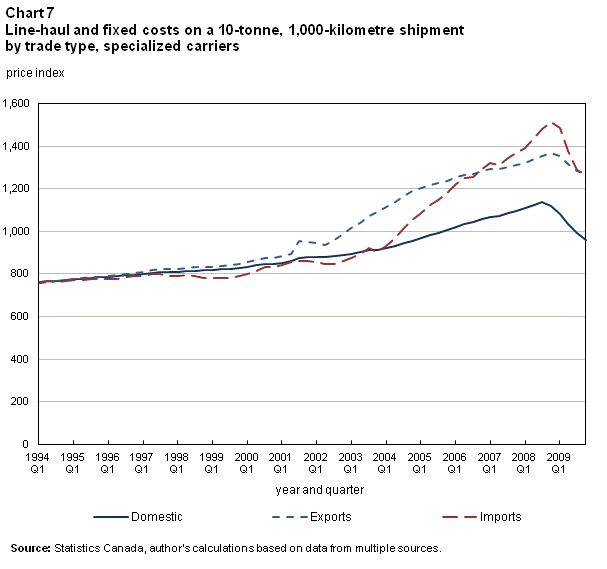
Charts 7 and 8 present the overall costs for specialized carriers and less-than-truckload carriers (see the appendix for the econometric estimates). For specialized carriers, fixed costs on exports do rise during the third quarter of 2001 and during the period leading up to 2004. While fixed costs follow a different pattern for specialized carriers than for truckload carriers, the pattern for line-haul costs is essentially the same, with rising relative line-haul costs on imports after 2004. The major difference with truckload carriers is that the gap between the price on exports and domestic shipments widens after 2001 and persists. For commodities shipped via specialized carriers, border thickening has not receded. For less-than-truckload carriers, there is some evidence of border thickening after 2001, because of rising fixed costs (Appendix Table 2).

A complete picture of border thickening requires that its effects for all types of carriers be brought together and that its contribution to the delivered price of goods be taken into account. The next section of the paper addresses both requirements.

Description for chart 7

Description for chart 8

4 Ad valorem trucking costs

To fully assess the question of border thickening and its persistence, it is necessary to abstract from measuring border costs based on level differences across carrier types and to move to measuring border costs on an ad valorem basis for all truck-borne shipments. This is tantamount to measuring the ad valorem tariff equivalent of the additional cost of moving goods across the Canada–U.S. border. A brief discussion follows on how these ad valorem costs were calculated and on their levels and trends.

4.1 Calculation of ad valorem costs

Ad valorem trucking costs require a measure of the value of goods shipped, which the Trucking Commodity Origin and Destination (TCOD) Survey does not supply. Hence, the value of each shipment has to be imputed using estimates of the value per tonne by commodity. In previous work (see Anderson and Brown [2012]), estimates of the value per tonne were derived from U.S. sources (i.e., the North American Transborder Freight Database (TFD) and the Commodity Flow Survey). In the interim, new Statistics Canada data have become available that provide estimates of value per tonne at a much more detailed commodity level and so these data were adopted.

In 2008, experimental transaction-level import and export files were developed to provide estimates of the tonnage of each shipment, in addition to its value. Shipments are coded by transportation mode and by origin and destination, providing the value per tonne at the HS10 (Harmonized System) level for imports and at the HS8 level for exports.^{Note 16}

Using the value per tonne estimated for 2008, the nominal value per tonne was projected across the study period using import and export price indices.^{Note 17} In total, there were 148 export series and 211 import series, and these were linked to the export and import records via their related HS8/HS10 commodity codes.^{Note 18} The estimated HS commodity coded values per tonne were then concorded with the five-digit Standard Classification of Transported Goods (SCTG) and linked them to TCOD Survey files. Therefore, on a shipment-by-shipment basis, estimates of carrier revenues and of the value of the goods shipped are available.

The measure of carrier revenues and the value of goods shipped were used to calculate the ad valorem trucking costs for domestic trade, imports and exports. This was done for the within‑sample observations used in the econometric analysis above, because the model estimates are used in the analysis to follow, across all carrier types (truckload, less-than-truckload and specialized). These rates are then benchmarked to reflect the five-digit SCTG commodity composition of the full sample of the TCOD Survey^{Note 19} for domestic trade and the two-digit HS commodity composition of Canada–U.S. truck-borne trade reported by the TFD for exports and imports. Hence, as much as possible, the commodity composition of trade reflects known totals, and, therefore, ad valorem rates are reflective of the actual commodity composition of trade.

4.2 Ad valorem transportation cost tariff equivalents

Ad valorem trucking costs for domestic trade and exports and imports over the 1994 to 2009 period are presented in Chart 9. Domestic ad valorem costs run just under 1.5% though much of the period, but rise about half a percentage point between 2003 and 2004 to about 2.0% and remain at that level for the remainder of the period. Export and import ad valorem rates are always above domestic levels, with export rates above import rates until 2006. Of course, differences in the commodity composition of trade (which can influence the denominator and numerator of the ad valorem calculation) and the distance shipped are not taken into account when calculating these rates, making comparisons across trade types problematic.

Description for chart 9

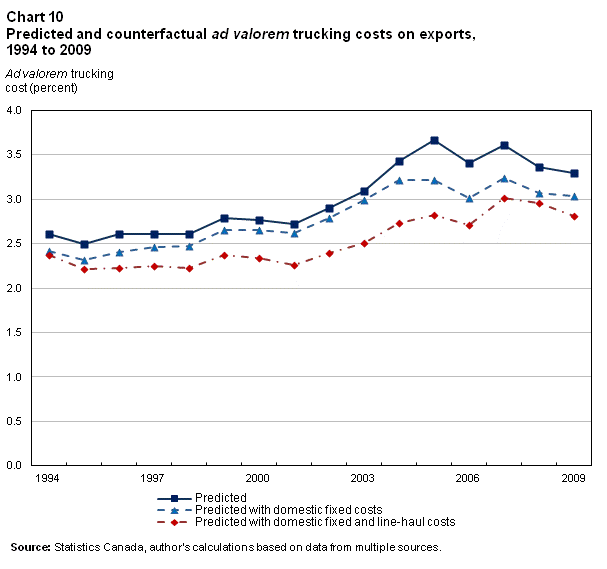
To control for differences in the distance and commodity composition of trade, ad valorem rates for exports and imports were predicted using domestic fixed and line-haul costs, generating a counterfactual rate. The difference between the predicted ad valorem rates and the counterfactual ad valorem rates can be thought of as the tariff equivalent of the additional costs of crossing the border. Chart 9 reports the predicted ad valorem rates. These closely match the actual ad valorem rates, and, therefore, there is no loss of generality by using the predictions.

Predicted and counterfactual ad valorem rates for exports and imports are presented in Charts 10 and 11. On the export side, both higher fixed and line-haul costs contribute to the additional cost of U.S.-bound shipments, with rising fixed costs after 2004. Once again, fixed costs do not rise immediately after 2001. However, it is noteworthy that after 2001 line-haul costs grow at a more modest pace for domestic trade than exports. It may be that higher costs of moving goods to the United States are being incorporated into line-haul rates, rather than being a fixed surcharge per shipment. On the import side, of primary interest is the effect of rising line-haul costs relative to domestic costs after 2004. It is only during this period that the gap between domestic rates and import rates opens up.

Description for chart 10

Description for chart 11

As noted above, the difference between the predicted ad valorem rates and the counterfactual rates, based on domestic fixed and line-haul costs, is the ad valorem tariff equivalent of moving goods across the border. Before discussing the tariff equivalents, it is useful to consider the relationship between the export and import series.

Depending on the circumstances, the two series may be negatively or positively correlated. They tend to be negatively correlated because the prices charged on the export and import legs of a round trip are tied. Firms have to commit capacity to both legs when they take a contract for one, and so the price charged on one leg of the journey depends negatively on the demand for the other. This means that the additional costs of shipping across the border may not be borne on the leg for which they are incurred, but on the leg for which the relative demand is the greatest (the fronthaul) (see Felton [1981]). The lesson to be learned is that in a world where the fronthaul and the backhaul switch between the export and import legs, it is best to look at the mean of the tariff equivalent on exports and imports to address the question of whether the border is thickening and, if so, whether this thickening persists (see the dashed line in Chart 12).

The two series are positively correlated if they share a common demand or supply shock. That is, they move together if there is some common shock shifting the export–import round-trip supply curve or demand curve. After the late 1990s, Canada–U.S. trade was not rising rapidly, and so a rightward shift in the demand curve is unlikely. Instead, there was a potential supply shock resulting from new border compliance measures and from increased delays (or variability in delays) at the border, which could have caused the supply curve to shift leftwards, pushing up prices on both the import and export legs.

Two expectations follow from this basic analysis. The first expectation is that import and export tariff equivalents should diverge when there is a shift towards an imbalance in export and import trips. Based on Chart 3, there are two periods of imbalance: (1) between 1998 and 2002, when export trips outweigh import trips (imports = backhaul), and (2) between 2005 and 2009, when import trips outweigh export trips (exports = backhaul). The second expectation is that, between 2001 and 2005, import and export tariff equivalents should move upwards in tandem as the industry reacts to a common supply shock driven by an increase in the cost of moving goods across the border.

Chart 12 shows that, early in the period, the tariff equivalents on imports and exports essentially match each other, with rates between 0.2% and 0.4%. Consistent with expectations, the ad valorem tariff equivalents on exports and imports diverge after 1997, with the rates on exports about double those on imports by the early 2000s. Between 2002 and 2005, the ad valorem tariff equivalents on exports and imports move upwards in tandem. This was a period when increased delays at the border and additional border compliance costs would have pushed the supply curve for both imports and exports to the left.^{Note 20} After 2005, the tariff equivalents on exports and imports once again move in opposite directions, falling for exports and rising for imports. This was also the period during which the relative demand for the import leg of the round trip rose steadily relative to the export leg.

Finally, border thickening can be seen best when looking at the mean of the tariff equivalents on exports and imports. Its value remains essentially unchanged between 1994 and 2002, before rising steadily between 2002 and 2005, after which there is once again little change, but which remains at a level well above the average between 1994 and 2002. This is clear evidence of border thickening and its persistence. Over the period from 1994 to 2000, the average of the import–export mean tariff equivalent was 0.33%, while, between 2005 and 2009, the average was 0.62%.

Of course, if competition for cross-border trips declined over the same period, then rising rates might not be attributable to border thickening. There is, however, little evidence that this occurred. Taking advantage of the fact that the interaction term between tonne-kilometre and tonnes $(\omega )$ is a measure of competition,^{Note 21} for truckload carriers there is no significant difference between $\omega$ for domestic shipments and for exports and imports (see Table 2).

It is important to keep in mind that while the ad valorem tariff equivalent is relatively small, the premium on cross-border ad valorem rates is significant. Between 1994 and 2000, it cost on average 16.2% more to ship goods across the border than to ship the same goods the same distance domestically, with no trend upward or downward. After 2000, the premium rose steadily to 25.1% in 2005 and stayed relatively high thereafter. And, depending on the period and the leg of the cross-border trip, the premium can be larger still. In 2005, the premium on the export leg was 30.0%, and the premium on the import leg had risen to 25.6% in 2009.

It should also be kept in mind that many goods pass back and forth across the border several times as they move through various stages of the production process. This is especially true of automotive supply chains (Andrea and Smith 2002). Car parts pass over the border up to six times before the final product is sold to consumers.^{Note 22} At each stage of the production process value is added. Goods for which relatively little value is added at a particular stage are the most sensitive to border thickening. Take a $100 item that is composed of $90 worth of intermediate inputs, and, by subtraction, $10 of value was added. In 2005, the additional cost of shipping this item to the United States over the pre-2001 level was about 0.5%, or $0.50. This is a small amount. However, this additional cost is 5% of value added, which could easily be the firm’s profit margin. Therefore, in the case of goods for which each step in the production process adds a small amount of value, the additional costs of shipping goods to the United States loom much larger.

Description for chart 12

5 Conclusion

The purpose of this paper is to identify the costs of trucking goods across the Canada–U.S. border from 1994 to 2009. This is a period marked by substantial changes in the Canada–U.S. trading relationship. It stretches from the final phasing-out of tariffs under the North American Free Trade Agreement, through the terrorist attacks on 9/11 that ushered in a new security regime that continues to evolve, to a substantial rise in the Canadian dollar after 2002. These changes had potentially two countervailing effects on the rates charged on exports to the United States in the post-9/11 era. The new post-9/11 security regime put upward pressure on rates, while the changing relative demand for export and import trips switched the backhaul from the import to the export leg of the round trip.

At the micro level, there is evidence that border compliance costs are reflected in prices. Through most of the period, fixed costs per shipment were higher for exports than for domestic trade. After 2001, fixed costs rose more rapidly for exports, but much of this rise occurred after 2003 and coincided with new border regulations. It was also after 2003 that line-haul costs of exports rose at a slower pace than those of imports and domestic trade, which is consistent with the switch in the backhaul from the import to the export leg of the cross-border trip.

When measured on an ad valorem basis, there is evidence of border thickening. After 2002, the ad valorem tariff equivalent of crossing the border rose for both the import and export legs of the cross-border round trip. This was the only period when these rates moved in tandem, suggesting a common supply shock. From 2005 onwards, the ad valorem tariff equivalents for exports and imports moved in opposite directions, but their mean remained the same. That is, the rising cost of moving goods across the border that occurred during the early to mid-2000s persists, but the burden of these extra costs has switched from the export to the import leg of the cross-border trip.

The costs measured here are only part of the total cost of shipping goods across the border. Institutional costs borne by exporting firms (e.g., customs administration) can be as great as or greater than costs passed on in the form of higher trucking prices (Taylor, Robideaux and Jackson 2004). Furthermore, variability in crossing times can add to the costs of exporters. This uncertainty can be hedged by adding buffer times into shipping schedules, which should be reflected in carriers’ revenue. Alternatively, exporters may choose to maintain buffer inventories on the other side of the border, which add directly to their costs (Anderson and Coates 2010).

Appendix

Notes