
Publications
Economic Analysis Research Paper Series
The Distribution of Employment Growth Rates in Canada: The Role of High-growth and Rapidly Shrinking Firms
The Distribution of Employment Growth Rates in Canada: The Role of High-growth and Rapidly Shrinking Firms

Archived Content
Information identified as archived is provided for reference, research or recordkeeping purposes. It is not subject to the Government of Canada Web Standards and has not been altered or updated since it was archived. Please "contact us" to request a format other than those available.

by Jay Dixon and Anne-Marie Rollin
- Abstract
- Executive Summary
- 1 Introduction
- 2 Background
- 3 Data and measures
- 4 Distribution of employment growth rates in Canada
- 5 Contributions of high-growth firms and rapidly shrinking firms to aggregate growth
- 6 Quantile regression framework
- 7 Quantile regression results
- 8 Conclusion
- 9 Appendix
- Notes
Abstract
This paper uses data from Statistics Canada's Longitudinal Employment Analysis Program database to study the distribution of annual employment growth rates in Canada over the 2000-to-2009 period, with a special emphasis on firms in the tails of the distribution, referred to here as high-growth firms (HGFs) and rapidly shrinking firms (RSFs).
The study has three objectives. First, it describes the distributions of employment growth rates in Canada to see whether they are consistent with observations in other countries. Second, it quantifies the contribution of HGFs and RSFs to aggregate job creation and destruction. The third objective is to examine, using quantile regression techniques, the role of firm size and firm age in the performance of HGFs and RSFs.
The results show that, as in other countries, the distributions of employment growth rates in Canada have more density both in the centre and in the tails than a normal distribution. While most firms do not change their employment much year-on-year, those that grow or shrink rapidly account for a large share of employment created and destroyed every year. Finally, small firm size is a more important predictor than age for RSFs, while age of the firm, specifically younger firms, is a better predictor of HGFs than size. Smaller firms of any age are more likely to shed a large proportion of their employment year-on-year, whereas younger firms of any size are more likely to post high annual growth rates.
Executive summary
Popular discussions of firm growth focus on stories of rapid increase and decline. Empirical studies of firm dynamics, by contrast, focus on average or representative, firm growth. Using standard econometric techniques such as linear regression, they examine how firm characteristics such as size and age affect the central tendencies of growth distributions. These techniques either ignore or are augmented to minimize the influence of rapidly growing and shrinking firms. However, because these firms may be responsible for a substantial amount of the economy’s employment dynamics, minimization is inappropriate.
This paper explores the contribution to net employment growth of high-growth firms (HGFs) and rapidly shrinking firms (RSFs) using Statistics Canada’s Longitudinal Employment Analysis Program (LEAP) data. After describing the distribution of employment growth rates, it asks whether HGFs and RSFs are, indeed, disproportionately important for understanding employment creation and destruction in Canada from 2000 to 2009. It then examines the influence of firm characteristics, specifically industry, firm size and firm age, in fostering high growth or rapid decline.
The LEAP dataset has advantages over data used in other studies of firm growth. Most datasets are limited in their coverage of firms by industry or by size, but LEAP covers all Canadian employer firms. More important, whereas most studies examine total firm growth, including the transfer of jobs through mergers and acquisitions, the structure of LEAP makes it possible to isolate net creation or destruction of employment—organic growth—at the firm level.
The study finds that the distribution of firm growth is peaked around zero, but has more density in the extremes than the normal distribution. The shape of the distribution reflects the fact that most firms exhibit little organic growth, regardless of industry, size or age. On the other hand, a small number of firms with very high rates of employment growth or destruction account for a disproportionate share of the overall employment dynamics in the Canadian economy. Quantile regressions reveal that age is a factor in high growth: regardless of size, younger firms are more likely to post high growth rates. Size, by contrast, is a factor in the probability of decline, with smaller firms being more likely to shrink rapidly.
This paper makes three contributions to the literatures on firm growth. A large body of research examines average growth patterns. This study demonstrates that the average tendencies of Canadian firms are driven by the tails of the growth distribution, which is consistent with findings for other countries.
The study's other contributions are to relate not only high growth, but also rapid decline, to firm characteristics using quantile regression techniques. A growing literature on HGFs and related literatures on gazelles and entrepreneurship study firms in the positive tail of the distribution. This research usually resorts either to case studies of particularly prominent firms, or to defining arbitrary growth thresholds and describing the average characteristics of firms exceeding them. RSFs, on the other hand, have largely been neglected. The present study uses quantile regression to examine the characteristics of firms along the entire distribution of growth outcomes, including HGFs and RSFs, without the need to define arbitrary growth thresholds.
1 Introduction
In 1999, a small unknown start-up Internet company moved its eight employees from a garage to new offices. By 2004, Google was no longer a start-up and no longer unknown. It was also no longer small, having increased its workforce to 3,021 employees. In 2010, it had 24,400 full-time employees worldwide, and a year later the number was 32,467.1
The rise of Canada’s Research In Motion (RIM) was not as meteoric, but the company still managed annualized average employment growth of over 35%, growing from 200 employees in 1998 to 17,000 in 2012.2 Another Canadian high-tech firm, Nortel, followed a different path, reducing its 90,000-strong workforce by an average of 17% a year from 2000 to 2005, before filing for bankruptcy at the end of the decade.3
Stories of rapid growth and decline typify popular discussions of firm growth. The rise of companies like Google and RIM, and the decline of Nortel, have made these firms household names. Their experiences have also visibly transformed their industries.
As important to the economy as these firms seem to be, they present a challenge to researchers. Most studies of firm dynamics look at central tendencies of growth distributions. Using techniques such as linear regression, they examine how firm characteristics such as size and age affect firm growth on average. But these statistical techniques either ignore or are augmented to minimize the influence of firms like RIM and Nortel.
Yet because such firms may be generating a substantial amount of the employment dynamics being studied, minimization seems inappropriate. The firms that are the most interesting in terms of innovation and productivity-enhancing resource allocation are probably not among the average performers. Rather, they are among the firms that are growing or shrinking rapidly: the firms in the tails of the growth distributions.
An increasing literature on high-growth firms (HGFs) and related literatures on gazelles and entrepreneurship attempt to identify and analyze firms in the positive tail of the distribution. These literatures usually resort either to case studies of particularly prominent firms, or to defining arbitrary growth thresholds and describing the average characteristics of firms that exceed them. Although both approaches reveal details about the growth process, they are not a substitute for rigorous statistical analysis.
Furthermore, little research has been devoted to firms that markedly downsize—labeled rapidly shrinking firms (RSFs) in this study. Indeed, the literature on HGFs and gazelles does not have a clear left-tail parallel. However, “creative destruction” as initially described by Schumpeter (1942) emphasizes the importance of the destructive process. Established firms are constantly being challenged by young innovative firms, and must sometimes dramatically adjust their workforce in response.
Based on Statistics Canada’s Longitudinal Employment Analysis Program (LEAP) data for 2000 through 2009, this paper explores the entire distribution of annual employment growth of Canadian firms. Whereas most datasets are limited in their coverage of firms by industry or by size, LEAP data encompass all employer firms in Canada. More important, most studies examine total firm growth, including the transfer of jobs through mergers and acquisitions, but the structure of LEAP makes it possible to isolate net creation or destruction of employment—organic growth—at the firm level.
This paper shows that the distributions of Canadian firms’ employment growth rates are not Gaussian: they have more density in the centre and in the tails than the normal distribution. The thicker-than-normal tails raise two questions.
First, how important are the firms in the tails of the distribution to overall employment growth? Although firms exhibiting very high growth or very rapid decline are more numerous than expected, do they contribute disproportionately to aggregate employment dynamics in Canada?
Second, a large body of research examines whether average growth patterns depend on firm size and firm age. This study asks how firm size and age affect the growth prospects of firms away from the average. Does size or age have any bearing on the propensity to be an HGF or an RSF? In particular, are larger firms more stable than smaller firms? Do smaller/younger firms tend to be more growth-oriented?
The next section reviews the empirical literature on firm growth distributions, including the tails. Section 3 explains the data source and the empirical measures used. Section 4 describes the distribution of employment growth in Canada. Section 5 presents results on the contribution of HGFs and RSFs to overall employment dynamics. Section 6 introduces the quantile regression model used, and Section 7 presents the results of these regressions. Section 8 concludes.
2 Background
This study draws on three bodies of literature: an extensive one on firm growth that goes back more than half a century; a much smaller one on the nature of firm growth distributions primarily associated with the econophysics research field and a burgeoning literature on high-growth firms.
2.1 Firm growth
The literature on the determinants of firm growth is too extensive to chronicle here. Much of it centres on the validity of Gibrat’s Law—Robert Gibrat’s 1931 observation that firms’ expected growth rates are independent of their size. Sutton (1997) is the most cited discussion of the theoretical implications of Gibrat’s Law. Audretsch et al. (2004) provide the most comprehensive meta-study of existing empirical work; of the 59 studies they list, 31 find that the “Law of Proportionate Growth,” as Gibrat’s Law is also known, is violated in one way or another.
Gibrat’s Law suggests that the distribution of shocks that firms face is independent of their size and their capacity to respond is proportional to their size. If true, the observed distributions of growth rates, conditional on size, have identical means and variances, and do not exhibit persistence.
Many studies find a negative relationship between average firm size and growth, which contradicts Gibrat’s Law. Others do not. For example, recent studies by Dixon and Rollin (2012) and Haltiwanger et al. (2010) of the Canadian and U.S. economies, respectively, find that in the 2000s, any negative relationship between size and growth that does exist disappears, and in fact becomes positive, when firm age is taken into account.
Most studies have found that the variance of growth rates is negatively related to size, suggesting that smaller firms are at greater risk of decline or failure and/or have greater opportunities to grow.4 This finding is intuitively appealing. Small firms are thought to have a tenuous relationship to financial markets, which amplifies the effects of shocks. Moreover, larger firms usually have a broader portfolio of products to buffer them against demand shocks. However, Sutton (2002) finds that the relationship between firm size and volatility is flatter than would be expected, suggesting that financial market access and portfolio diversification provide some, but not much, additional stability.
The literature does not address how much of the greater volatility of small firms is due to moderate but frequent shocks and adjustments, and how much is due to less frequent but much larger changes in firm employment. It also implicitly assumes that the distributions of growth rates are symmetric—small firms are equally more likely to advance/decline than are larger firms.
2.2 Firm distributions
Most of the literature on firm growth has looked only at the first (mean) and second (standard deviation) moments of growth. Studies of the overall shape of firm growth distributions are less common and have been undertaken with European data by Bottazzi and Secchi, and with American data by “econo-physicists,” a small group of physicists applying the tools of their discipline to firm-level micro-data. These studies reveal a tent-shaped distribution in the growth rates of firm employment, sales and assets for large American firms in the Compustat data (Amaral et al., 1998; Stanley et al., 1996); the worldwide pharmaceutical industry (Bottazzi and Secchi, 2005); Italian manufacturing (Bottazzi et al., 2007); Chilean manufacturing (Halket, 2006); and French manufacturing industry at various levels of disaggregation (Bottazzi et al., 2011). Lothian (2006) also found a tent-shaped distribution of the annual growth of Canadian firms' sales for 1976 to 1998.
Their presence in so many datasets, and their persistence at various levels of aggregation, make tent-shaped distributions a stylized fact that theories of firm growth must accommodate. Some explanations note the similarity between firm growth distributions and those of phenomena in the natural sciences, but these models are difficult to explain via variants of economic behaviour.
Stanley et al. (1996) propose a model in which firms are composed of multiple units, each of which grows or shrinks according to Gibrat’s Law. As each unit grows, it becomes harder to manage, making it increasingly appealing to split off some of its resources to start a new unit, leading to a large jump in firm size. While this explanation seems plausible for the large firms in their data (they use Compustat data, which cover only large, publicly traded U.S. firms), it seems less appropriate to describe small firms as being composed of units. Yet other studies show the same distributions for smaller firms.
Coad and Planck (2012) offer a more general model, based on the concept of self-organizing criticality. Firms are able to grow because of a certain amount of organizational slack that managers seek to minimize. Additional production workers can be integrated into the hierarchy of a firm as long as there are enough supervisors to manage them. At certain critical points, supervisory resources become too stretched, and incorporating more workers requires the hiring of new supervisors, which, in turn, requires new managers, human resources specialists, and so on. Small shocks are thus capable of generating large changes in firm size.
It is also possible that the distributions are an artifact of the data. Halket (2006) suggests that growth rates appear to follow variance gamma (also called generalized Laplace) distributions. They arise when the magnitude of change is stochastic and follows a normal distribution, and the timing of the change is also random and follows a gamma distribution. In the case of firms, it suggests that employment is subjected to shocks of random sizes, occurring at what appear in the data to be random times. Firms may, indeed, be making changes with uncertain outcomes, but according to a predetermined plan. The schedule of those changes will be determined by a variety of details specific to the product sold, the technological process used, and other industry- or even firm-specific factors. Data collection, on the other hand, typically follows a schedule set by the sun: employment data, for example, are collected on a specific calendar date, or if not, are calendarized after the fact. The appearance of random timing could thus reflect a discrepancy between calendar and “economic” time.
2.3 Firms in the tails
2.3.1 High-growth firms
Research on distributions has mainly focused on a growth process that is common across firms. Nonetheless, an expanding literature argues that firms in the positive tails—HGFs—differ from other firms. HGFs are credited with being uniquely important to economic growth, as job creators and drivers of innovation. The popular conception of HGFs is that they are high-tech start-ups bringing revolutionary technology to the economy.
However, the HGF literature has not generated a cumulative evidence base, largely because studies use different datasets, indicators of growth, and definitions of high growth. The result has been confusion about the nature and significance of the high-growth process. One interpretation of this confusion is that firm growth in general, and high growth in particular, is a heterogeneous phenomenon with different types of firms following different paths to growth.
Because “all high-growth firms do not grow in the same way,” Delmar et al. (2003) argue that studies based on single growth measures will be informative about only one type of organizational growth. Studies of sales or asset growth may paint a different picture of the process than do studies of employment. Research on total growth, including mergers and acquisitions, may identify different firms as HGFs than does research examining organic growth alone, with very different implications. Similarly, it has been argued that absolute changes may paint a different picture than relative measures.
Most studies use a single growth measure. Delmar et al. (2003, p. 194) note “an emerging consensus that if only one indicator is to be chosen as a measure of firm growth, the most preferred measure should be sales.” However, the majority of HGF studies have focused on employment. One reason may simply be that early researchers were preoccupied with job creation. But if firms are viewed as collections of resources, employment may be a better measure of a firm’s size and complexity than the value of its products.5
Henrekson and Johansson (2010) provide an extensive survey of studies of HGFs as job creators. They examine three propositions about the nature of HGFs: 1) they are over-represented in high-tech industries; 2) they are younger than other firms; and 3) they are smaller than other firms. Henrekson and Johansson conclude that HGFs are found in all industries, not just in high-tech, and while they are relatively young and small, they are not all start-ups. In fact, they may not necessarily be all that young: Acs et al. (2008) find that the average age of high-impact firms was 25 years.6 Also, large HGFs contribute significantly to job creation in absolute terms.
Henrekson and Johansson (2010) note the problem of defining HGFs, and the studies they cite use different definitions. The definition of 20% average annualized growth over three consecutive years from Eurostat and the Organisation for Economic Co-operation and Development (Eurostat and OECD, 2007)7 is the most common, but other thresholds and time periods are used. Some research looks at the top fraction of firms by growth, like the top 5% or 10% fastest-growing firms. Both definitions are arbitrary.
Studies also differ in whether their HGFs grow “organically” (adding new jobs) or also by mergers and acquisitions (taking existing jobs from other firms). Firms that grow organically add more employment through the labour market, or sales by directly cultivating new customers. Firms expanding through acquisitive growth, on the other hand, add new employees or customers by merging with or acquiring other firms. Because of data limitations, most work on HGFs has studied total growth—organic and acquisitive together.
From the firm’s perspective, both organic and acquisitive growth lead to an expansion in the resources they need to manage. But from a social perspective, organic and acquisitive growth have different implications. If the social objective is to expand the number of jobs, then studies should focus only on organic growth. Acquisitive growth, in and of itself, does not create net employment but rather, transfers existing jobs from one firm to another. Also, acquisitive and organic growth may be at odds in terms of their social significance. McKelvie and Wiklund (2010) find that acquisitive HGFs are often organic destroyers of jobs.
Evidence suggests that the mode of growth differs systematically across types of firms. Studies in Sweden (Delmar et al., 2003) and Finland (Deschryvere, 2008) find that growth in young and small firms tends to be organic, while larger and older firms are more likely to grow through acquisition. Delmar et al. (2003, p. 210) conclude: “In relation to previous research, these results largely support a view that organic growth is more associated with young and small firms, and that acquisition growth is more common among larger and older firms, and firms in stagnant or low-tech industries.”
Most studies use percentage growth, although some use absolute growth or combinations of the two. Because many studies of firm growth start from Gibrat’s Law, relative growth tends to be more popular, though some authors argue that absolute growth is more appropriate for answering the question, “Who creates jobs?” In the context of HGFs, some studies caution that because it is easier for smaller firms to achieve very high growth rates, even if they are adding few employees, relative measures may be misleading.
This paper looks exclusively at year-on-year organic growth. It also focuses on relative growth, which is often suspected of giving an advantage to smaller firms in terms of being identified as “high-growth.” However, the results in Section 7 suggest that this “small base problem” may not be a major issue. This study does not set arbitrary criteria for identifying HGFs.
2.3.2 Rapidly shrinking firms
Research has been conducted on the determinants of exit, or equivalently survival, but the same type of statistical analysis has not been applied to firms that reduce their workforce severely. According to various studies, young age and small size increase a firm’s probability of going out of business (Geroski, 1995; Evans, 1987; Baldwin, 1995; Mata and Portugal, 1994; Esteve Perez et al., 2004).
What factors contribute to pronounced downsizing? Currently, the literature does not provide an answer to this question, although a few studies have looked at growth patterns in the years before exit (Troske, 1996; Huynh and Petrunia, 2012). But while some shrinking firms perform poorly before exit, others remain competitive by drastically diminishing their workforce. It may be that small and/or young firms slim down rapidly in the face of negative shocks because of limited financial resources. On the other hand, stories of well-established mature firms laying off many employees as part of a restructuring strategy are common.
Simultaneously studying the right and left tails of the growth distribution, as is done in this study, serves to more fully delineate the nature of the competitive process.
3 Data and measures
3.1 Data source
This analysis uses information from Statistics Canada’s Longitudinal Employment Analysis Program (LEAP),8 an administrative database that includes all firms in the Canadian economy that have some payroll, and therefore, issue at least one “Statement of Remuneration Paid” (a T4 slip). It covers incorporated and unincorporated businesses, but excludes self-employed individuals and partnerships in which the participants do not draw salaries. It is a longitudinal file, which means that the employment level of firms is tracked over time on an annual basis.9
The LEAP file covers only organic growth. It removes “spurious” births and deaths of firms that can arise from corporate restructuring, for example, mergers and acquisitions (M&A), spinoffs, and divestitures. These transactions represent jobs changing firms rather than the creation of new jobs or the destruction of existing jobs, which is the process examined here.
False births and deaths are removed through “labour-tracking.” Clusters of employees of appearing and disappearing firms are compared to the clusters of employees of other firms in the previous year (for appearing firms) or the following year (for disappearing firms). If a substantial portion of employees is found previously or subsequently in another firm, a connection is made between the two firms involved, and the structure of the firm in year is applied to the data of both firms in year and all preceding years.
The LEAP database comes in vintages. When an additional year of data becomes available, a new longitudinal file, or vintage, is created. LEAP vintage 2009 tracks firm employment from 1983 to 2009; vintage 2008 tracks employment from 1983 to 2008, and so on. Each vintage holds the structure of the firm constant using information for the most recent year available. For example, LEAP vintage 2009 aggregates all earlier annual data based on the firm’s structure in 2009; vintage 2008 aggregates earlier data based on its structure in 2008. Thus, two firms that merge in 2009 are considered to be a single firm from 1983 to 2009 in the 2009 vintage, but are recorded as separate firms from 1983 through 2008 in the 2008 vintage.
The advantage of this treatment is that it abstracts almost completely from plants changing hands, recording only “organic growth" due to the addition of new plants or new employees at existing plants. The LEAP database is thus able to isolate firm activity that changes the economy’s demand for labour.
However, the fact that each vintage pushes the market structure of its last year back in time creates an extra challenge. For each vintage, pushing the current structure further back beyond risks misclassifying the sources of growth for every year except the last two. For example, the structure in the 2007 vintage of a firm that was involved in M&A activity in 2008 is clearly different from the structure in the 2009 vintage. It is not the case that the merged firm, as it exists in year , can be held responsible for the consolidated operations in year of the separate firms from which it was formed.
This paper deals with the misclassification problem in earlier years of each vintage by using only data from the last two years of each LEAP vintage from 2000 to 2009. The result is a series of ten cross-sections, which are pooled to study the distribution of growth rates. This reduces the comparisons to one-year periods, with the firm structure held constant for the second year of each cross-section.
This study is restricted to the business sector. This is done by excluding the cross-sections classified in the North American Industry Classification System (NAICS) sectors 91 (public administration), 61 (education services) and 62 (health care and social assistance).10
3.2 Measuring firm employment and age
The LEAP database contains annual payroll information (total payroll and total number of workers who received a T4 slip over the calendar year). Based on these data, firm employment is inferred through a measure called the Average Labour Unit (ALU).11
The ALU measure divides each firm's annual payroll by the average annual earnings of a representative worker in the same industry, province and firm size class, determined using data from Statistics Canada’s monthly Survey of Employment, Payrolls and Hours.12 For a description of the ALU calculation, see Lafrance and Leung (2010).
The ALU is a proxy for employment. It can vary along two dimensions—the number of workers and their average remuneration. The latter differs across firms because of longevity of employment over a year, hours worked, and wages paid. While firms with a small ALU may have fewer employees, and larger ones may have more, firms may also appear large because they pay higher wages than the industry average, or small, because they pay less. This measure, therefore, takes job quality, as measured by wages, into account.
When firms are active for only part of the year, their employment is underestimated by the ALU measure. This underestimation is more important for start-ups created at the end of the calendar year, and for exits that close down in the first months of the year. Underestimation of the size of entries and exits has implications for growth rates in the year after entry, and in the year before exit. Growth rates of start-ups that survive into the next year are overestimated, and growth rates between the year before exit and the exit year are more negative than they actually were. Because of this data limitation, only incumbent firms that are at least two years old are included in this analysis.13
A firm age is assigned to every cross-sectional record, using the methodology described in Dixon and Rollin (2012).
3.3 Defining firm size and growth rate
The standard “average-year" methodology outlined by Davis et al. (1996) is used to calculate firm size and growth rate for each cross-sectional observation . Firm size, denoted , is the average size of the firm in years and . This is written as:
The growth rate of cross-sectional observation from year to year is defined as:
where is the firm employment in year , and is its employment in year .
This formulation ameliorates the effects of short-term regression to the mean—the tendency of growing (declining) firms to go back to their mean employment level in the next period by downsizing (increasing) their workforce.
The growth rate used yields similar results to log growth rates, at least for firms expanding or contracting employment by up to 50% (by log-average measures). The chief difference with log growth is that the “average-year" growth rate is linear and bounded between -2 (exit) and 2 (entry) at the extreme ends. As a result, entries and exits make up a distinct subset that is not directly comparable to other observations. In addition, the size attributed to these cross-sectional observations corresponds, by construction, to half the actual size of the firm upon entry or exit. Because of the arbitrary treatment of entry and exit, this analysis focuses on continuing firms, which represent the base of firms active across two consecutive years.
Incumbents for which is below one ALU are also excluded because of the small-base problem. In such cases, infinitesimal changes in employment can result in very high or very low growth rates.
4 Distribution of employment growth rates in Canada
4.1 Overall distribution
As discussed in Subsection 2.2, the distributions of firm growth rates observed in various countries have been found to be non-Gaussian, with more density in the centre and the tails. To illustrate the distribution of employment growth rates for Canadian firms, histograms are constructed by creating bins of growth rates of 0.05, or approximately 5% (log) in length, and calculating the share of observations in each bin. The width of the bins was chosen to preserve firm confidentiality and simplify the exposition.
The distribution of employment growth rates for incumbent firms varied only slightly across the 10 years studied even though the period included the economic recession of 2008-2009 (Chart 9 in Appendix). Pooling observations for all these years is, therefore, the methodology adopted in the remainder of the paper.
The empirical distribution differs substantially from a normal distribution (Chart 1). It is a leptokurtic distribution in that it is peaked in the centre and has thicker tails.
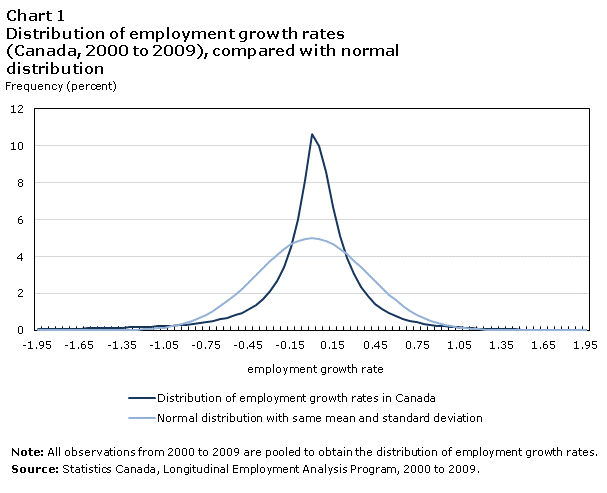
The central tendency of the distribution, as measured by the mean and the median, is close to zero (see text box below). This, and the tight concentration of density around the centre, imply that most firms do not change their employment much year-on-year. Half the firms—those between the 25th and 75th percentiles—alter their employment by less than 15% on either side.
| Number of observations: | 5.3 million |
| Mean: | -0.02 |
| Standard deviation: | 0.40 |
| Skewness: | -0.75 |
| Kurtosis: | 4.86 |
| 10th percentile: | -0.43 |
| 25th percentile: | -0.15 |
| Median: | 0.00 |
| 75th percentile: | 0.15 |
| 90th percentile: | 0.36 |
| Interquartile range: | 0.30 |
| Interdecile range: | 0.78 |
The distribution is skewed to the left. This negative skewness manifests itself in a skewness statistics of -0.75, and also in the mean (-0.02) being lower than the median (0.00). Therefore, the mean is influenced by the density in the left tail, which is fatter than the right tail.
Kurtosis, which measures the peakedness and the end-tail thickness, is 4.86. This is greater than the normal (3.0), but lower than the Laplace distribution (6.0). A d’Agostino-Pearson normality test was performed and rejected the null hypothesis of a Gaussian distribution, both on the basis of asymmetry and excess kurtosis.
Altogether, this evidence paints a picture of firm growth dynamics whereby a large number of firms change very little each year, and a small number grow or decline markedly.
The shapes of the distributions are not what would be expected from firm growth that consists of a large number of independently distributed innovations.14 They resemble generalized Laplace distributions, which are sometimes used in finance for pricing options. The prices of these options are known to experience frequent jumps or spikes that are difficult to model using independently and identically distributed normal random variables. That firm growth follows similar distributions suggests that firms can be also prone to discontinuous rather than smooth change.15
4.2 Conditional distributions
4.2.1 Industry
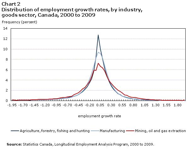
Charts 2 and 3 depict firm growth distributions conditional on industry. As mentioned in the introduction, the popular conception is that HGFs are concentrated in high-tech industries. If true, it would imply that the distribution for the industry categories containing the high-tech industries (especially manufacturing) should have thicker tails than other industries.
In fact, the thickness of the tails, where the candidates for HGFs and RSFs reside, is common to all industries. That is, although rapid growth and rapid decline are popularly associated with the high-tech industry, the outcomes of most other industries have the same Laplace-like distribution. This is in line with the high-growth literature, which reports the presence of HGFs in various industries (Henrekson and Johansson, 2010).

4.2.2 Size and age
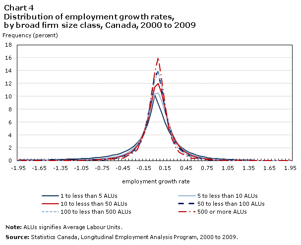
Much of the literature on firm dynamics centers on the relationship between size and growth, sometimes accounting for firm age. As noted in Section 2, the literature is ambivalent as to whether Gibrat’s Law holds for means, but routinely finds larger variance in growth rates for smaller firms.
The results of the present analysis suggest that the differences in conditional means and variances by firm size are driven not by the mass of firms in the centre of the distribution, but by the firms in the tails. In particular, the tails of the distribution are thicker for smaller size classes, especially for firms with fewer than 10 employees (Chart 4). But the influence of size seems to be asymmetrical: the negative tail gets thicker faster than the positive tail as firm size decreases.
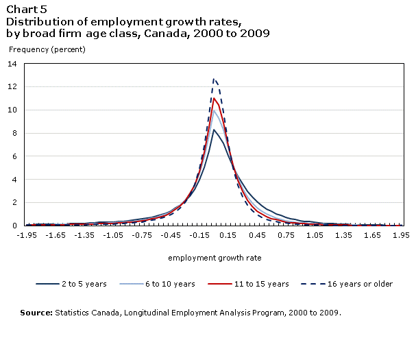
The growth distributions of younger firms have thicker tails than do older firms (Chart 5). But the age distributions exhibit the opposite asymmetry to the size distributions. The positive tail is especially thick for younger firms.16 The positive skew of these distributions suggests that, unlike their older counterparts, younger firms either tend to be high growing, or to have already exited (in which case, they are not in the data).
These findings raise a number of issues. First, the non-Gaussian nature of the distributions of firm growth rates requires an explanation, but this is left for future research. Second, how much do firms in the tails of the distribution contribute to overall employment dynamics? Section 5 explores their contribution to aggregate job dynamics.
Third, although much of the literature on firm dynamics looks at firms’ expected growth based on characteristics such as size and age, the differences between various types of firms are most pronounced in one or both tails. Section 6 investigates how the shapes of the distributions vary by firm size and age, using quantile regression methods.
5 Contributions of high-growth firms and rapidly shrinking firms to aggregate growth
The results of the previous section show that employment varies only slightly in most continuing firms, but fluctuates substantially in the small number of HGFs and RSFs. But which firms are responsible for most of the employment dynamics—the large number of firms making small changes, or the small number making large changes?
About one million employers are active every year in the Canadian business sector. Figures 1 and 2 present the contributions of different types of firms to gross employment creation and destruction. These tables distinguish between incumbents and entry/exit. A separate category displays incumbent firms that are one year old and/or have less than one ALU. This category raises some concerns. The employment growth of one-year-old firms is likely overestimated owing to the ALU methodology. Most firms are active for only part of their entry year, which results in underestimation of entry size, depending on the date of entry. Micro-firms (less than one ALU) suffer from the small-base problem, which tends to inflate their growth rate.

Note: Figure 1 shows that three groups of firms contribute to gross employment creation. Entries contribute 19%. Incumbents one year old and/or of size less than one contribute 13%. Finally, incumbents two years old or older and of size one or larger contribute 68%. high-growth firms (HGFs) studied in this analysis belong to the third group of firms, which are also called established growing incumbents. When HGFs are defined as having a growth rate of 20% or higher, which is the case for the top 18% of established growing incumbents, they account for 47% of total gross employment creation. When HGFs are defined as those established growing incumbents with the top 10% growth rates, the cut-off growth rate is 35%, and the group accounts for 38% of total gross employment creation.
Source: Statistics Canada, Longitudinal Employment Analysis Program, 2000 to 2009.
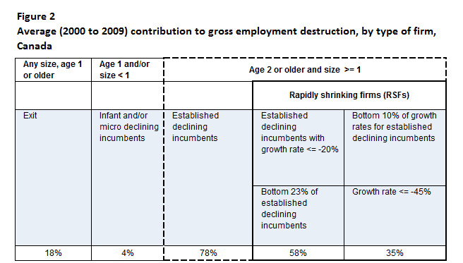
Note: Figure 2 shows that three groups of firms contribute to gross employment destruction. Exits contribute 18%. Incumbents one year old and/or of size less than one contribute 4%. Finally, incumbents two years old or older and of size one or larger contribute 78%. rapidly shrinking firms (RSFs) studied in this analysis belong to the third group of firms, which is also called established declining incumbents. When RSFs are defined as having a rate of decline of 20% or smaller, which is the case for the bottom 23% of established declining incumbents, they account for 58% of total gross employment destruction. When RSFs are defined as those established declining incumbents with the bottom 10% growth rates, the cut-off growth rate of decline is 45% and the group accounts for 35% of total gross employment destruction.
Source: Statistics Canada, Longitudinal Employment Analysis Program, 2000 to 2009.
Of the approximately half million firms that contribute to employment creation every year, established incumbents (aged two years or older and with at least one ALU) are responsible for two-thirds of new employment. On the destruction side, established incumbents account for more than three-quarters of employment losses. The bulk of employment dynamics, therefore, occurs among established incumbents.
However, within this category, most employment changes are generated by the fastest growers and decliners. HGFs and RSFs can be defined two ways: using a quantile cut-off or using a growth-rate threshold. When HGFs are defined as firms with an annual growth rate of 20% or more (which make them candidates for HGF designation according to the OECD definition of 20% average annualized growth over three years), they account for only 18% of established growing incumbents, but are responsible for nearly half of employment creation. The top 10% fastest growers, that is, firms above the 90th percentile (growth rate of 35%), account for almost 40% of overall employment creation.
The contribution of RSFs to employment destruction is similarly disproportionate. Based on a rate of decline cut-off of 20%, which is in line with the OECD definition, 58% of destruction is accounted for by the bottom 23% of decliners. The bottom 10% of decliners, those that shrink at a minimum rate of 45% per year, are responsible for a third of annual employment destruction.
Regardless of how HGFs and RSFs are defined, firms in the tails of the growth rate distribution are clearly important drivers of employment dynamics in Canada. What firm characteristics are better predictors of very high growth and decline?
6 Quantile regression framework
The previous sections have shown that the distributions of firm growth rates do not comply with the assumptions of standard regression models. Moreover, the results suggest that studying firms in the tails, rather than in the centre of the growth distribution, is the key to understanding employment dynamics in Canada.
These findings create problems for standard statistical techniques. The skewed and heavy-tailed nature of the distributions means that standard estimates of the relationship between growth and firm characteristics such as size and age must be interpreted cautiously. Outliers can skew estimates of conditional means, and kurtosis affects standard errors used for inference. Insofar as there is systematic variation across different firms in higher moments, they will distort conclusions about average tendencies.
As well, standard methods are geared toward central tendencies, and are thus ill-suited to incorporate information at other points in the distribution, namely, the tails. Studies of HGFs typically deal with this problem by defining an arbitrary growth threshold, and then analyzing the average characteristics of the firms that exceed it.
This paper opts instead to use quantile regression. This technique has the advantage of being non-parametric, which means that inference is not affected by the shape of the underlying distribution. In addition, with quantile regression, it is possible to examine the relationship between firm characteristics and, say, high growth, directly without relying on arbitrary thresholds.
Much of the literature on firm employment dynamics has looked at firm size and age as explanatory variables, asking whether small firms grow faster than larger firms after controlling for other factors. The present study asks whether smaller (larger) firms are more likely to be high growth (rapid decline), or are more prone to shrink rapidly, and whether the relationship between high growth/rapid decline is affected by the age of the firm.
To estimate the statistical relationship between growth rates and age and size at various points in the distribution, the following regression model is used:
where the superscript means that the coefficient is evaluated at quantile . The index are size classes, and is an indicator function that equals 1 if firm belongs to the given size class in time . The count variable is defined as 17 minus the age of the firm, and takes the value of 0 for firms that are aged 17 years or older.17,18 The vector contains control variables (dummies for year and industry).
The omitted categories for the dummy variables are a middle-size class (20 to less than 50 ALUs), year 2003 and manufacturing (NAICS 31 to 33). Defining as years younger than the 17 or older age category is equivalent to excluding the oldest category.
Estimates were obtained for every fifth quantile, for a total of nineteen ( = 0.05, 0.10, ..., 0.95). Confidence intervals were generated using Markov chain marginal bootstrapped standard errors with 200 iterations. For details on the mechanics of quantile regression, see Koenker (2005) or Hao and Naiman (2007).
In the case of linear regression, the intercept corresponds to the mean growth rate of the omitted categories, and the coefficients on the dummy variables are the change in the mean that results from changing categories, holding other factors constant. For quantile regression, the intercept is the growth rate of firms defined by the omitted categories (firms with at least 20 but less than 50 ALUs and aged 17 years or older) at a point in the distribution specified by . The coefficients are the differences in growth rates at percentile between the reference group and firms in size class , controlling for age and other characteristics. The coefficients and can be used to calculate the marginal impact of being one year younger (older) on growth of firms at quantile , controlling for size and other characteristics.
7 Quantile regression results
Firms that experience high growth or that shrink rapidly are a prominent feature of the data, and are quantitatively significant contributors to aggregate growth dynamics. But what types of firms are most likely to be high-growth or rapidly shrinking? The main regression results in Charts 6 to 8 concentrate on two characteristics: firm size and age.
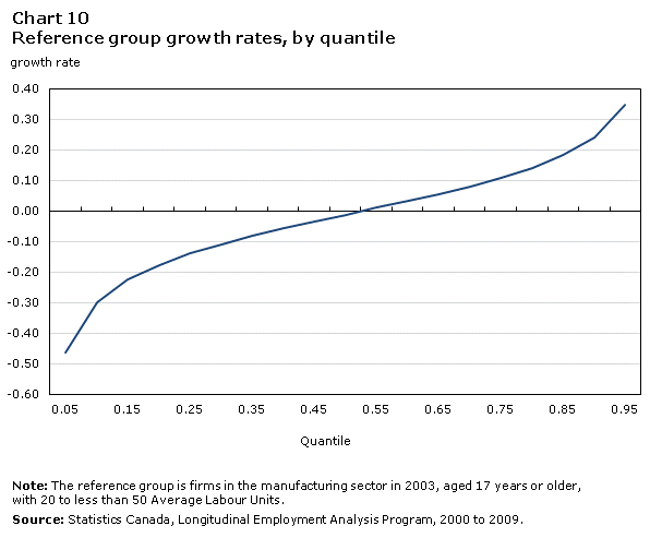
Charts 6 and 7 plot the size class coefficients for firms smaller and larger than the reference group (firms with 20 to less than 50 ALUs), respectively. Growth rates for the reference group are normalized to zero, and therefore line up on the horizontal axis. Chart 10 in the Appendix shows growth rates of the reference group.
The lines in Charts 6 and 7 represent how much faster (values above the horizontal axis) or slower (values below the horizontal axis) a given size class grows compared to the reference group in every quantile. Positively (negatively) sloped lines signify that the size class has greater (less) dispersion than the reference group: more (less) negative growth rates in the left tail and more (less) positive growth rates in the right tail.
Skewness manifests itself in a difference in the distance from the horizontal axis between the left and right sides of the median. Negative skewness means that firms are more likely to shrink rapidly than to grow rapidly, while positive skewness indicates greater upside potential. If the left-hand side is further from the horizontal axis than the right-hand side, the distribution is negatively skewed. Alternatively, if the right-hand side is further than the left-hand size, then the distribution is positively skewed.
With regards to firm size, four results stand out. First, median growth rates, ( =0.5, marked by a diamond in the charts) tend to be lower for firms smaller than the reference group (Chart 6), and higher for firms larger than the reference group (Chart 7). The median growth rates are statistically different from one another for smaller size classes, but not for larger size classes. That is, when controlling for age, industry and time effects, a positive relationship emerges between size and median growth for firms below a middle-size threshold but there is no relationship for firms above the threshold. These results for the conditional medians confirm the findings of Dixon and Rollin (2012) and Haltiwanger et al. (2010) for the relationship between mean growth and size.
The second observation is that while the relationship between median growth and size is statistically significant for the smaller size classes, there is quantitatively not much difference in median growth rates across all size classes. Firms with 5 to less than 10 ALUs grow only fractionally more slowly than do the firms in the 20-to-less-than-50-ALU reference group, and even firms with 1,000 or more ALUs grow only slightly faster than the reference group (less than 0.01 difference in growth rates).
The third finding is that the main difference between firms in different size classes lies not with median firms, but with firms that are growing or shrinking rapidly. Charts 6 and 7 show that the growth of small firms is more volatile than that of larger firms. The 10% most rapidly shrinking firms with less than 5 ALUs shrink 22% more rapidly than their counterparts in the reference group, and the top 10% (quantile 0.90) grow 6% more rapidly. Chart 7 shows that the most rapidly shrinking larger firms have growth rates that are less negative than corresponding firms in the reference group, while the highest growing ones post growth rates that tend to be less positive.
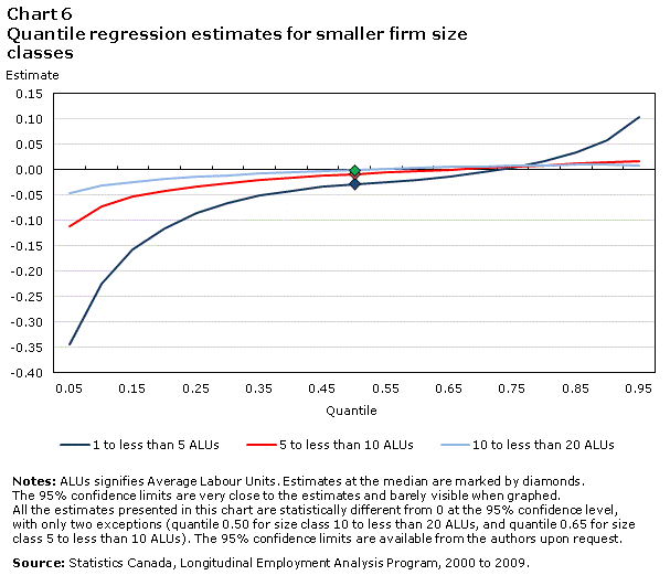
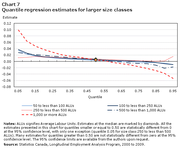
Finally, the impact of size on the growth of firms in the tails is negatively skewed, meaning that size has more significant implications for rapidly shrinking firms than for high growth firms. The distance from the horizontal axis for the lowest quantiles is larger than for the highest quantiles. All the estimates for the 25th percentile are statistically different from zero, but this is not true for estimates at the 75th percentile. There is a relationship between firm size and the 25% left-tail growth rate cut-off (the smaller the firm, the more negative the 25th percentile growth rate), but no such relationship is apparent on the high-growth portion of the distribution. Smaller firms are more prone to shrink rapidly, as can be seen from the large distance to the horizontal axis for the lowest quantiles. As size increases, growth rates at the lowest quantiles are less negative.
In summary, there is a slight positive relationship between firm size and typical growth experience for smaller firms. But the main difference between firms of different sizes is that small firms are more volatile. Furthermore, this volatility comes less from a greater probability of being an HGF, and more from small firms’ greater risk of negative outcomes. One possible explanation is that small firms are less able than large firms to insure themselves against negative shocks. Alternatively, if negative shocks are correlated, shrinking firms are more likely to be small.
The patterns for age are opposite to those for size. Because firm age is a count variable, the coefficients and can be used to estimate the impact of a firm getting one year younger or older. Chart 8 plots, for selected ages, the marginal effect of various quantiles, which is calculated from the estimated coefficients:
can be interpreted as the difference in growth at quantile from surviving one additional year from a given age.
Chart 8 shows that surviving another year reduces the volatility of growth rates, at all ages. The impact of age is right-skewed—for very young firms especially, an extra year of age does more to reduce the growth rates of the highest growers than it does to slow the decline of the most rapidly shrinking firms. Firm aging does not affect substantially median growth rates, where most firms are located.
The impact of firm aging flattens out, and becomes more symmetrical as firms increase in age. Becoming one year older makes less than 1% difference in growth rates either way for firms aged 15 or older.

From Chart 8 it is hard to see the cumulative effect of many extra years of age. Table 1 presents the growth rates predicted by the regression model for selected size and age categories. It reveals pronounced differences between firms aged 2 and 15 years located in the tails of the distribution. For the quantiles presented ( = 0.05, 0.10, 0.25, 0.50, 0.75, 0.90 and 0.95), the absolute difference at all size classes between these two age groups is 0.23, 0.14, 0.02, 0.04, 0.14, 0.25, and 0.33, respectively. For example, for the 20-to-less-than-50-ALU reference size, the median predicted growth rate is 0.03 for firms aged 2 versus -0.01 for firms aged 15. The corresponding numbers for the 10th percentile are -0.45 and -0.31, and 0.50 and 0.25 at the 90th percentile. The difference is larger in the right tail than in the left tail, and negligible in the centre of the distribution.
Together, the quantile regressions suggest that size and age make minimal differences to year-on-year organic employment growth for most firms—those in the centre of the distribution. However, these characteristics do matter for RSFs and HGFs.19 Firms become more stable as they get older and larger. The most important differences are that smaller firms at any age are more prone to shrink rapidly than larger firms, while younger firms are more likely to be HGFs compared to older firms.
8 Conclusion
This study explores the distribution of firm growth rates in Canada from 2000 to 2009. It finds that the distributions of Canadian employment growth rates are non-normal or non-Gaussian. Consistent with findings for other countries, they have more density both in the centre and in the tails than a normal distribution. The distributions suggest that, year-on-year, most firms change very little, but a minority grow or shrink rapidly.
The second observation is that the firms in the tails are an important feature of Canadian employment dynamics, accounting for a large share of jobs created and destroyed in the past decade.
The third contribution of this paper is its examination, using quantile regression techniques, of the role of size and age in the performance of firms in the tails. Haltiwanger et al. (2010) and Dixon and Rollin (2012) show that the apparent negative relationship between size and average employment growth disappears when age is added as an explanatory variables in ordinary least squares (OLS) regressions.
However, the results presented here suggest that neither characteristic is particularly useful to distinguish among firms in the middle of the distribution—the relationships between employment growth and age and size are more pronounced in the tails. But they are asymmetric: small size is more important than age for RSFs, while age, or more precisely being a young firm is a better predictor of HGFs.
The results have a number of implications for the literature. First, the lack of a strong relationship between size and the growth of the typical firm in Canada from 2000 to 2009 suggests that average results are influenced by atypical firms. It raises the prospect that the ambiguous results on size and average growth reported in the literature for other countries, industries and time periods may reflect the specific characteristics of HGFs and RSFs in the samples used.
Second, the literature has found a negative relationship between firm size and the variance of growth. The results here confirm such a relationship for Canadian firms. However, the greater variance for smaller firms comes predominately from negative risks, whereas positive risk is an inverse function of age.
The study suggests that a richer understanding of firm dynamics requires looking beyond first and second moments. Future research will concentrate on how the higher moments of distribution of firm growth rates differ across industries and over the economic cycle.
9 Appendix

Notes
- Numbers for Google are from http://www.google.com/about/company/history and from Google Annual Reports for 2004, 2010 and 2011, which are available at http://investor.google.com\pdf\2004_google_annual_report.pdf; http://investor.google.com\pdf\2010_google_annual_report.pdf; and http://investor.google.com\pdf\2011_google_annual_report.pdf .
- Numbers for Research In Motion are from its 1998 and 2011 Annual Reports, which are available at http://www.rim.com/investors/documents/pdf/annual/1998rim_ar.pdf and http://www.rim.com/investors/documents/pdf/annual/2011rim_ar.pdf .
- Numbers for Nortel are from its 2008 Annual Financial Statements (http://www.nortel-canada.com/wp-content/uploads/2011/11/2008_nnc_annual_financial_statements.pdf) and its 2005 Annual Report (http://www.sec.gov/Archives/edgar/data/72911/999999999706021043/9999999997-06-021043-index.htm).
- Stanley et al. (1996) suggest that the relationship between variance and size may, in fact, be governed by a power law with a slope between -0.17 and -0.21 for large American firms. Bottazzi et al. (2011) find a similar relationship for French manufacturing firms, but Bottazzi et al. (2007) find no relationship between size and variance for Italian manufacturing firms. By contrast, Perline et al. (2006) find a slight positive relationship between size and variance for a sample of small American firms.
- For the theory of firms as collections of resources, see Penrose (1959).
- The authors define high-impact firms as firms that have at least doubled their sales in a four-year period, and have had high absolute and relative employment growth.
- Estimates that use multiple years of growth are often used to deal with regression to the mean, which is common in firm-level datasets.
- See Baldwin et al. (1992) for a description of the construction of the database.
- The administrative data in LEAP are structured at the level of the “statistical enterprise,” which is the level associated with a complete set of financial statements. For simplicity’s sake, this statistical unit is referred to as “the firm” in this study.
- In Canada, the education and health sectors are heavily financed by the public sector. Firms in the excluded sectors have different motives than firms in the business sector—they are not necessarily profit-maximizing.
- No direct measure of employment is available in LEAP—firm employment is imputed using annual payroll information.
- If a firm is present in multiple provinces, its national ALUs correspond to the sum of its provincial ALUs. Also, the same size class is used in all provinces, because firm size is considered to be a national characteristic. However, the dominant industry for a given firm is allowed to change across provinces.
- Excluding exiting incumbents a year before exit would require using three consecutive years of data.
- According to the Central Limit Theorem (CLT), a large number of independently distributed shocks should result in a normal, or Gaussian, distribution, regardless of the exact distributions that produce them, provided that none of the shocks is dominant and all have finite variance.
- For details on Laplace distributions and the stochastic processes that generate them, see Reed (2007).
- Charts 4 and 5 were also done with narrower size and age classes. The same tendency was observed—the tails are heavier for smaller and younger groups.
- The maximum age that can be consistently identified for all years studied is 16 years.
- Similar results to those in this paper were obtained using a regression model with dummy variables using age ranges instead of a count variable.
- Quantile regressions were run for the goods and services industries separately, using the same model used in this paper. A comparison of the results revealed no differences in the patterns between the two sectors.
- Date modified: