
Analytical Studies Branch Research Paper Series
The impact of firm closures and job loss on participation in gig work: A causal analysis
Skip to text
Text begins
Abstract
This study uses data from the Statistics Canada Longitudinal Worker File linked to Canadian census records to examine the impact of firm closures and involuntary job loss on entry into gig work. The analysis distinguishes between the actions of those who experienced an actual layoff associated with a firm closure and those who worked in a closing firm but did not necessarily wait until the closure (“impending layoff”). The results show that job displacement associated with firm closures roughly doubles the probability of entry into gig work in the year of displacement and the following year.
Keywords: gig work, independent contractor, layoff, job displacement, exact matching, difference-in-difference
Executive summary
Much of the rapidly growing literature on the gig economy has so far focused on identifying gig workers, documenting their characteristics and measuring the size of the gig economy. With very few exceptions, the literature is still mostly descriptive, and some key questions such as “Why do individuals become gig workers?” remain largely unanswered. This study dives deeper into the reasons why individuals enter informal work arrangements and examines the impact of involuntary job displacement caused by a firm closure on the probability of entry into gig work. It conducts a full-scale causal investigation of the impact of imminent and actual job loss on entry into gig work using a uniquely rich nationally representative database that combines longitudinal administrative data from multiple sources, including individual tax and employment records linked to firm-level data on firm closures. The administrative data are further linked to census microdata, which add essential information about the level of educational attainment and other individual characteristics usually unavailable in administrative files. The link between administrative and census data is unique in the literature on gig work.
The analysis differentiates between the effects of an actual permanent layoff (AL) and an impending (anticipated) permanent layoff (IL) on participation in gig work. The IL analysis examines the possibility that some workers proactively leave the closing firm, and this may impact the probability of becoming a gig worker. The strategy used to identify gig workers in the administrative data is the same as in Jeon et al. (2021). The gig worker category consists of unincorporated self-employed individuals with weak expectations of future continuity and less predictable future earnings, such as freelancers, independent contractors and consultants, and on-demand online platform workers. The study points out that, although gig workers are viewed in this study as a subset of unincorporated self-employed individuals, it is a distinct group, whose entry into gig work is likely to be governed by a different set of considerations than entry into self-employment more generally.
The main data source in this study is the Longitudinal Worker File (LWF), a large administrative database designed to provide information about employment dynamics in Canada. Annual T1 and T4 files form the basis of the LWF, providing detailed data about individual earnings and income sources. However, the LWF contains only basic demographic information such as an individual’s age, sex, marital status and area of residence. The LWF records are linked to 2016 Census records to obtain additional information on individual characteristics.
The study covers the period from 2008 to 2015. Among all individuals who satisfied certain conditions, those who worked in firms that closed in year and were present in that firm at any time during were identified as members of the treatment group for the IL analysis. Among them, individuals who also experienced a permanent layoff in were identified as members of the treatment group for the AL analysis. Individuals who satisfied the same pre- restrictions as the treatment group but neither worked in firms that closed in nor experienced any job displacement in were designated as the control group. Coarsened exact matching was used to balance the observed characteristics of the treatment and control groups. The matched sample was then used to estimate the differences in the probability of being a gig worker between the treatment and control groups in three post- years.
In the AL analysis, the study found that the probability of being a gig worker was about 48.6% higher in the treatment group than in the control group in the year following the year of the firm closure (). The effect gradually faded away in subsequent years, but the probability of being a gig worker was still 33.8% higher for the treated than the controls in . In the IL analysis, the probability of being a gig worker in was 24.5% higher for the treatment group than the control group. These results seem to indicate that those who had remained with the closing firm until the end were substantially more likely to do gig work later than those who had left the firm before the closure, either because their post-layoff earnings were lower than they had been before the firm closure and they needed to supplement their income or because they were unable to find suitable reemployment.
Among displaced workers who entered gig work in the year of the firm closure (), more than half (54.9%) were still doing gig work the next year. Different patterns of gig work participation were observed for displaced workers with different levels of educational attainment. For university degree holders, the effect in was large, but it diminished in subsequent periods and became small and not statistically significant in . For those with less than a high school education, the initial effect in was not very large, but it was larger in than in .
The results also suggest substantial cross-industry differences in the magnitude and the duration of post-closure effects. Workers displaced from manufacturing firms or retail firms were substantially more likely to be engaged in gig work than the control group, but the numbers of individuals observed in gig work in other industries were generally too small for the results related to these industries to be conclusive. Finally, younger workers (aged 25 to 34 years) were notably less likely to engage in gig activities following a firm closure than workers older than 45, and particularly those aged 55 to 59. Possible explanations for this result include the relative scarcity of reemployment opportunities for older workers compared with younger ones and also lesser geographic and occupational mobility often required for reemployment.
1 Introduction
Much of the rapidly growing literature on the gig economy has so far focused on identifying gig workers, documenting their characteristics and measuring the size of the gig economy (Abraham & Houseman, 2019; Abraham et al., 2018, 2019; Bracha & Burke, 2021; Collins et al., 2020; Garin et al., 2020; Jackson et al., 2017; Jeon et al., 2021; Katz & Krueger, 2017; Kostyshyna & Luu, 2019; Koustas, 2020; Mas & Pallais, 2020). With very few exceptions, the literature is still mostly descriptive, and some key questions, such as “Why do individuals become gig workers?,” remain largely unanswered.
This study dives deeper into the reasons why individuals enter informal work arrangements and examines the impact of involuntary job displacement caused by a firm closure on the probability of entry into gig work. Based on the evidence accumulated so far, there are good reasons to suspect that job loss is an important determinant of entry into gig economy. Katz and Krueger (2017) reported a positive relationship between unemployment and working in an alternative work arrangement a year later. Jackson (2019) examined short- and long-term consequences of taking up gig work by unemployment insurance recipients and noted that earnings generally decline before entry into gig work. Koustas (2019) and Garin et al. (2020) documented a considerable drop in average individual earnings right before entry into gig work using US administrative data. Jeon et al. (2021) documented a similar drop in earnings and increase in the probability of receiving employment insurance (EI) benefits before entry into gig work using Canadian administrative data. Workers who quit their job or are dismissed for misconduct are usually not eligible for EI benefits in Canada, so a spike in the probability of receiving EI benefits suggests that entry into gig work is often precipitated by permanent layoffs. However, neither the US studies nor Jeon et al. (2021) made any causal inferences regarding the impact of job loss on entry into gig economy.
This study conducts a full-scale causal investigation of the impact of imminent and actual job loss on entry into gig work using a uniquely rich nationally representative database that combines longitudinal administrative data from multiple sources, including individual tax and employment records linked to firm-level data on firm closures. The administrative data are further linked to census microdata, which add essential information about the level of educational attainment and other individual characteristics usually unavailable in administrative files. The link between administrative and census data is unique in the literature on gig work.
The analysis differentiates between the effects of an actual permanent layoff and an impending (anticipated) permanent layoff on participation in gig work. To analyze the effect of an actual layoff, the empirical strategy in this study is similar to the empirical strategy used in previous studies examining the impact of job displacement on entry into self-employment (Von Greiff, 2009) and measuring the earnings of displaced workers (Couch & Placzek, 2010; Hijzen et al., 2010). This strategy uses permanent layoffs caused by plant closures (or massive downsizing) as a proxy for exogenous job loss and compares post-layoff outcomes of displaced workers with the outcomes of matched controls who did not work in closing firms. At the core of this strategy is the assumption that workers laid off from closing firms “lose their jobs due to a reason beyond their control” (Couch & Placzek, 2010, p. 573), which minimizes the problem of selection into job displacement since less productive or less skilled workers have a higher probability of being laid off from partially downsizing firms than more productive and more skilled ones. This selection issue is important because productivity and skills are usually unobserved by researchers, which makes it difficult to identify appropriate counterfactual workers to measure the causal effects of job loss on the outcomes of interest.Note In this study, the effect of actual permanent layoffs is referred to as the actual layoff (AL) analysis.
However, this type of analysis implicitly ignores the possibility that workers are often aware of the impending closure and can take actions before the firm actually closes. Instead of waiting for the firm to close, more productive and higher-skilled (or better-connected) workers may be able to leave the firm and take a job elsewhere. This job transition is a consequence of the imminent firm closure, but the “proactive” workers who leave the firm because they anticipate its closure are not considered “treated” in the layoff analysis because no actual layoff is observed. Yet, the possibility of workers proactively leaving the closing firm is important in the context of an analysis of entry into gig work because many such job transitions are involuntary and the quality of the new employer–employee match may be lower, which may also result in lower earnings and contribute to workers’ decision to enter gig work. To shed light on how all involuntary job transitions may impact the probability of becoming a gig worker, this study turns to the intention-to-treat (ITT) framework.Note An essential element of the ITT framework is that all those assigned the treatment are considered treated regardless of whether they actually receive the treatment or not. In the context of this study, working in a closing firm is interpreted as having been assigned the treatment (permanent layoff), which means that all those working in soon-to-close firms and facing a potential layoff become members of the treatment group regardless of whether they are actually laid off when the firm closes or have left the firm some time before its imminent closure. The analysis based on the ITT framework will be referred to as the impending layoff (IL) analysis.
Among other important novel elements of the study is a discussion of theoretical considerations related to entry into gig work. The study argues that, although gig workers can be viewed as a subset of a larger category of unincorporated self-employed individuals, their entry into gig work is likely to be governed by a different set of considerations than entry into self-employment more generally. The study also recognizes the uncertainty surrounding the term “gig worker,” and in addition to identifying gig workers using the methodology proposed in Jeon et al. (2021), it also looks at the post-displacement decisions to become independent contractors, a subset of unincorporated self-employed workers identified through their business deductions (Lim et al., 2019).
The key finding of the AL analysis is that displaced workers have an almost 50% higher probability of being a gig worker in the year following the displacement year than similar workers in the control group who did not work in closing firms. Displacement roughly doubles the probability of a new entry into gig work in the year following the displacement year. However, the effect is substantially smaller in the IL analysis, which takes into consideration workers’ actions in anticipation of an impending firm closure.
2 Gig work and theoretical considerations related to entry into gig work
2.1 Who is a gig worker?
Despite the rapid growth of the economics literature on gig economy, there is no universally accepted definition of gig work, and different studies define gig work in different terms. It is generally understood that gig workers are individuals who enter short-term contracts to perform a particular task or to provide a specific service, often through online platforms (Abraham & Houseman, 2018; Boeri et al., 2020; Collins et al., 2020; Jackson et al., 2017; Katz & Krueger, 2017; Mas & Pallais, 2020). Such contracts are variably referred to as “informal work,” “alternative work arrangements,” “non-traditional work arrangements” or simply “gig work,” and individuals who enter them are contrasted with “traditional” employees whose work is covered by minimum wage laws, employment insurance, pensions and workplace safety regulations. Some gig work studies focus exclusively on individuals whose work is mediated by online platforms and view mediation provided by such platforms as the defining feature of gig economy (Donovan et al., 2016).Note Other studies see the growing online platform economy as an essential element, but not the only element of the widening spectrum of informal work arrangements, and base their definition of gig work on work characteristics rather than on how the relations between different labour market participants are mediated (Abraham et al., 2018; Jeon et al., 2021; Koustas, 2020).
Abraham et al. (2018) clarified many conceptual uncertainties related to the definition of gig work by introducing a typology of work arrangements and pointing out that work arrangements associated with gig work do not involve wages or salaries and are characterized by the lack of expectations of continuity and predictability of future earnings, work hours and work schedule. It follows that gig workers are a category of workers consisting of unincorporated self-employed freelancers, independent contractors and consultants, day labourers, and on-demand online platform workers. Importantly, the workplace characteristics of gig workers determine the way they report their income to the tax authorities. For instance, as self-employed individuals, they are expected to report self-employment income from business and professional activities, but not wages and salaries.
Using the typology of work arrangements in Abraham et al. (2018) as their conceptual guide, Jeon et al. (2021) developed an analytical strategy of identifying gig workers using Canadian tax data and introduced a method of measuring the size of the gig economy using an identifying strategy that was specific to the way unincorporated self-employed individuals report their earnings to the Canada Revenue Agency (CRA). Although there are similarities between the US and Canadian tax systems, there are also several essential differences discussed in Jeon et al. (2021). The key to their methodological strategy of identifying gig workers in Canada is information from Form T2125 Statement of Business or Professional Activities. Any unincorporated self-employed individuals, including online platform workers such as Uber drivers, are required to submit a Form T2125 with their individual tax returns (T1). However, the methodological strategy in Jeon et al. recognizes that not all unincorporated self-employed individuals reporting T2125 income are gig workers, so it also takes into consideration whether or not individuals submitting a T2125 indicate a business number (BN). The absence of a BN is taken to signal weaker expectations of future continuity and less predictable future earnings, and unincorporated self-employed workers who submit a T2125 with no BN are considered gig workers.
The Jeon et al. (2021) strategy of identifying gig workers is adopted in this study. However, this study also considers an alternative approach to identifying informal workers, similar to the one introduced in Lim et al. (2019) and discussed in detail in the Online Appendix to Jeon et al. (2021). Lim et al. (2019) referred to the category of informal workers identified in their study as independent contractors, and this study will maintain the same terminology differentiating between “gig workers” and “independent contractors.” Although both definitions attempt to capture a similar group of informal workers, such as independent contractors and freelancers, day labourers, independent consultants and platform workers, there is an important conceptual difference between them: while the gig worker definition is derived from workplace characteristics, the definition of an independent contractor is expense-based. The expense-based approach distinguishes between two categories of unincorporated self-employed individuals with T2125 income based on their business expense deductions: sole proprietors with T2125 income whose total expense deductions net of motor vehicle and travel expenses are below $15,000, and other unincorporated self-employed sole proprietors with T2125 income.Note The former category—T2125 sole proprietors with expense deductions under $15,000—is the category deemed “independent contractors.”Note
Jeon et al. (2021) found that 93% of those identified as gig workers were also identified as independent contractors, and among T2125 sole proprietors who were not identified as gig workers, about two-thirds satisfied the definition of an independent contractor. Hence, there was a large overlap between the two categories although the definition of an independent contractor appeared considerably more inclusive than the definition of a gig worker.Note A comparison between results obtained for gig workers and independent contractors should provide an important check of the sensitivity of the main results.
2.2 Theoretical considerations related to entry into gig work
Some of the clues regarding the role of job loss in the entry into gig work come from a much broader strand of the economics literature that examines motives and conditions for entry into self-employment. Simoes et al. (2016) provided a comprehensive overview of these studies noting various known determinants of entry into self-employment including age, marital status, family business experience and the availability of financial resources. Much of the discussion in the literature on entry into self-employment focuses on the relative importance of “push” factors leading to “necessity self-employment” versus “pull” factors leading to “opportunity self-employment” (Fairlie & Fossen, 2020). Job loss is usually identified as a “push” factor strongly associated with entry into self-employment. Farber (1999) was one of the first studies to find that alternative work arrangements, including self-employment, were highly prevalent among displaced workers. Krashinsky (2004) found that workers who had lost their jobs were two to three times more likely to become self-employed than those who had not. A carefully done Swedish study showed that displaced Swedish workers were almost twice as likely to be self-employed one year after the displacement as matched non-displaced workers (Von Greiff, 2009). Further evidence suggests that those who transition to self-employment from unemployment are more likely to be solo self-employed than those who transition from traditional wage employment (Boeri et al., 2020).
However, the importance of various factors affecting entry into gig work, including job displacement, should not be extrapolated from the existing evidence related to entry into self-employment. Although, as mentioned above, gig workers are usually viewed as a subset of unincorporated self-employed individuals, it is a distinct group, whose entry into gig work is likely to be governed by a different set of considerations than entry into self-employment more generally. One reason why entry into gig work may be driven by different considerations is that gig work does not usually require a large amount of capital investment.Note In the classic Evans and Jovanovic (1989) model, entry into self-employment is determined by differences between individual’s potential wages and salaries, , and self-employment earnings, , where is the market-determined wage, is the interest rate, is individual’s assets, is entrepreneurial ability, is a production function, is individual’s capital and is a random component of the production process. With a smaller capital investment required to maintain sufficiently high, liquidity constraints that would be binding for entry into more traditional form of self-employment may not be binding for entry into gig work. Not only does the relatively low bar for capital investment make entry into gig work easier, it may also attract a somewhat different group of entrants compared with those entering into more traditional forms of self-employment: those with different entrepreneurial or professional skills, different backgrounds, and different labour market prospects.
Another reason why entry into gig work may be driven by different considerations than entry into more traditional forms of self-employment is that, unlike the latter, gig work is often a side activity done to supplement earnings from traditional wage employment. In classic models of entry into self-employment, the choice between wage and self-employment is usually dichotomous (Evans & Jovanovic, 1989; Fairlie & Krashinsky, 2012). However, the literature on gig work has accumulated substantial evidence showing that many gig workers are also wage employees (Abraham & Houseman, 2019; Abraham et al., 2018 Bracha & Burke, 2021; Collins et al., 2020; Jeon et al., 2021). Jeon et al. (2021) found that about half of gig workers also receive wages and salaries. Even when displaced workers find new employment, they are likely to be employed at lower wages, and may still need to supplement their employment income with income from gig activities to maintain the pre-displacement level of consumption.Note
Although the existing evidence suggests that displacement may be an important determinant of entry into gig work, the causal impact of job loss on the probability of participating in gig work has not been formally established and the magnitude of the effect has not been quantified. Therefore, entry into gig work warrants a careful separate investigation.
3 Data and analytical sample
3.1 Data source and variable definitions
The main data source in this study is the Longitudinal Worker File (LWF), a large administrative database designed to provide information about employment dynamics in Canada.Note The LWF consists of several data components linked through unique individual and business identifiers, including individual tax returns (T1), Statement of Remuneration Paid (T4) files, Record of Employment (ROE) files, financial declaration (FD) files containing information from Statements of Business or Professional Activities (Form T2125), corporate tax return (T2) Schedule 50 files, and firm data from the Longitudinal Employment Analysis Program (LEAP).Note The LWF universe for a particular calendar year includes all individuals who either file a T1 for that year or receive at least one T4 slip in that year. This study uses LWF records from 2005 to 2016. Annual T1 and T4 files form the basis of the LWF, providing detailed data about individual earnings and income sources.
The LWF contains only basic demographic information such as an individual’s age, sex, marital status and area of residence. However, it is possible to link the LWF records to 2016 Census records to obtain additional information on individual characteristics. The 2016 Census microdata file is based on the long-form census questionnaire distributed to one in four Canadian households. Responding to the questionnaire is mandatory, and the 2016 Census microdata file is designed and processed to be representative of all Canadian households (Statistics Canada, 2019). Hence, the linked LWF–Census analytical data file is approximately a 25% random subsample of the initial LWF sample. Two main pieces of individual information were taken from the 2016 Census data: the highest level of educational attainment and immigrant status.
Firm closure. Information on firm closures comes from the LEAP component of the LWF. A principal advantage of the LEAP is that it uses employment tracking to identify firms’ mergers, acquisitions and “true deaths.” In the case of identifying the true death of firm , employment tracking involves identifying all employees before its potential death and locating their clusters in other firms. If any such cluster is identified in firm , the relationship between and is further investigated. If the two firms are found to be sufficiently similar, the death of firm is deemed false, and and are assigned a common longitudinal business identifier. The upshot of this process is that, in addition to containing important information about firm characteristics such as industry and firm size, the LEAP is particularly well suited for identifying true firm closures. For the analysis in the study, all firms that experienced exit from 2005 to 2015 were identified using LEAP data. For instance, if a firm existed in 2005 but did not exist in 2006, 2005 was deemed an exit year or the year in which the firm closed.Note
Displacement. Displacement information comes from the ROE component of the LWF. By law, Canadian employers have to submit ROE for all job separations occurring in their firms to the Canada Revenue Agency (CRA) since this information is used to establish workers’ eligibility for EI benefits. The ROE files contain detailed information about the reasons for separations, including “shortage of work,” labour dispute, illness or injury, quit and parental leave. ROE records are linked to LWF records to add information about all job separations occurring during a calendar year. An ROE record indicating a job termination resulting from shortage of work is deemed a permanent layoff if the employee does not return to the same firm in the year of the separation or the following year. Permanent layoffs resulting from firm closures can be identified by combining firm closure information from LEAP with permanent layoff data from ROEs using unique business and individual identifiers.
Gig workers and independent contractors. The key to identifying gig workers and independent contractors are FD files recently added to the LWF environment. These files, constructed by Statistics Canada, aggregate information on all individuals who report any positive gross self-employment income from farming, fishing, professional and business activities, commissions, and rental income to better suit analytical purposes. The FD variables related to professional, business and commission income correspond to the information from Form T2125, which, as mentioned in Section 2, plays a key role in identifying gig workers.
Owners of incorporated firms. In addition to unincorporated self-employed individuals, the LWF also allows for identification of owners of incorporated businesses. When a private corporation files a corporate tax return (T2), it also provides information about all shareholders with shares of 10% or more.Note This information, which comes from T2 Schedule 50 files, is attached to the LWF through unique personal identifiers and was used in this study to identify incorporated self-employed individuals.
3.2 Sample constructions and defining treatment and control groups
The empirical strategy for both the actual and impending layoff analyses is to compare post-treatment outcomes of workers from closing firms with the outcomes of similar workers from non-closing firms. This strategy is consistent with a more general framework of using matching methods for causal inference based on longitudinal data (Imai et al., 2021), and it consists of three essential steps: identifying the treatment and control groups with the same pre-treatment histories of the outcomes, matching treatment and control groups to make their observed characteristics as similar as possible, and using the matched sample to compute the estimands of interest in post-treatment periods by comparing the outcomes of the treatment group with the counterfactual outcomes of the control group.
The year in which a firm closes will be referred to as the treatment year () in both AL and IL analyses. In the IL analysis based on the ITT principle, it is assumed that the treatment is assigned on the first day of the treatment year () because the exact moment when individuals become aware of the impending firm closure and layoff is unobserved. Year is also the year in which members of the control group receive the “placebo treatment.”
Several restrictions on the analytical sample were imposed before defining the treatment and control groups. The first restriction established a three-year “washout” period, so that individuals who experienced any layoffs (permanent or temporary) or who worked in any firm that closed during the three-year period preceding were dropped from the sample. This was done to avoid the lingering effects of previous layoffs or firm closures on entry into gig work, since individuals could experience multiple permanent layoffs or work in multiple closing firms during a short time period.Note The second restriction required that all individuals had to work in the same firm for at least two consecutive years, and , therefore excluding individuals with very short tenures whose labour market behaviour and objectives may be different from those of the vast majority of workers. This condition also implicitly required that the closing firm existed in and excluded individuals who worked in firms that both entered and exited in . As in most other studies analyzing the impact of job displacement resulting from firm closures, individuals who worked in very small firms—fewer than five employees in —were also excluded from the sample because individual and firm exits in such firms are often intertwined. Lastly, the sample was restricted to individuals aged 25 to 59 in to focus on the labour market outcomes of the prime working-age segment of the population.
Among all individuals who satisfied the sample restrictions above, those who worked in firms that closed in , and were present in that firm at any time during , were identified as members of the treatment group for the IL analysis. Among them, individuals who also experienced a permanent layoff in were identified as members of the treatment group for the AL analysis. Individuals who satisfied the same pre- restrictions as the treatment group but neither worked in firms that closed in nor experienced any job displacement in were designated as the control group. For the IL analysis, the treatment group consisted of 79,450 unique individualsNote who worked in firms that closed during the 2008 to 2015 period . About one-quarter (24.3%) of them experienced a permanent layoff in according to ROE records, so the treatment group for the AL analysis consisted of 19,400 unique individuals.Note A small number of individuals in both treatment groups appeared in multiple treatment years () because these years were further apart than the three-year washout period: 501 individuals entered the treatment group twice in the IL analysis and 38 individuals did so in the AL analysis. Most individuals in the control group satisfied sample restitutions in more than one and therefore were used as controls for multiple . The control group consisted of 3,293,400 unique individuals contributing about 16 million observations from 2008 to 2015. The pre-matched sample characteristics are shown in Table 1 and discussed in the next section, which describes the matching algorithm that ensures balanced estimation samples.
| Actual layoff analysis | Impending layoff analysis | |||||||||||
|---|---|---|---|---|---|---|---|---|---|---|---|---|
| Pre-matched | Matched, coarsened exact matching weighted | Pre-matched | Matched, coarsened exact matching weighted | |||||||||
| Treated | Controls | Normalized differences | Treated | Controls | Normalized differences | Treated | Controls | Normalized differences | Treated | Controls | Normalized differences | |
| shares | normalized | shares | normalized | shares | normalized | shares | normalized | |||||
| Age at | ||||||||||||
| 25 to 29 | 0.133 | 0.122 | 0.032 | 0.132 | 0.132 | Note ...: not applicable | 0.158 | 0.122 | 0.104 | 0.158 | 0.158 | Note ...: not applicable |
| 30 to 34 | 0.138 | 0.134 | 0.011 | 0.136 | 0.136 | Note ...: not applicable | 0.145 | 0.134 | 0.032 | 0.145 | 0.145 | Note ...: not applicable |
| 35 to 39 | 0.136 | 0.137 | -0.005 | 0.135 | 0.135 | Note ...: not applicable | 0.136 | 0.137 | -0.004 | 0.135 | 0.135 | Note ...: not applicable |
| 40 to 44 | 0.138 | 0.144 | -0.018 | 0.138 | 0.138 | Note ...: not applicable | 0.138 | 0.144 | -0.019 | 0.138 | 0.138 | Note ...: not applicable |
| 45 to 50 | 0.164 | 0.162 | 0.007 | 0.164 | 0.164 | Note ...: not applicable | 0.152 | 0.162 | -0.026 | 0.153 | 0.153 | Note ...: not applicable |
| 50 to 54 | 0.161 | 0.166 | -0.014 | 0.163 | 0.163 | Note ...: not applicable | 0.151 | 0.166 | -0.041 | 0.152 | 0.152 | Note ...: not applicable |
| 55 and older | 0.131 | 0.134 | -0.011 | 0.131 | 0.131 | Note ...: not applicable | 0.119 | 0.134 | -0.045 | 0.119 | 0.119 | Note ...: not applicable |
| Female | 0.446 | 0.513 | -0.135 | 0.444 | 0.444 | Note ...: not applicable | 0.501 | 0.513 | -0.025 | 0.501 | 0.501 | Note ...: not applicable |
| Marital status at | ||||||||||||
| Couple | 0.622 | 0.674 | -0.111 | 0.629 | 0.629 | Note ...: not applicable | 0.629 | 0.674 | -0.095 | 0.636 | 0.636 | Note ...: not applicable |
| Single | 0.375 | 0.322 | 0.111 | 0.370 | 0.370 | Note ...: not applicable | 0.368 | 0.322 | 0.096 | 0.363 | 0.363 | Note ...: not applicable |
| Missing | 0.003 | 0.003 | -0.002 | 0.001 | 0.001 | Note ...: not applicable | 0.003 | 0.003 | -0.004 | 0.001 | 0.001 | Note ...: not applicable |
| Place of residence at | ||||||||||||
| Atlantic provinces | 0.066 | 0.069 | -0.011 | 0.065 | 0.065 | Note ...: not applicable | 0.081 | 0.069 | 0.046 | 0.080 | 0.080 | Note ...: not applicable |
| Quebec (except Montréal) | 0.123 | 0.133 | -0.030 | 0.124 | 0.124 | Note ...: not applicable | 0.104 | 0.133 | -0.090 | 0.104 | 0.104 | Note ...: not applicable |
| Ontario (except Toronto) | 0.206 | 0.216 | -0.024 | 0.208 | 0.208 | Note ...: not applicable | 0.180 | 0.216 | -0.090 | 0.182 | 0.182 | Note ...: not applicable |
| Prairies | 0.141 | 0.180 | -0.104 | 0.143 | 0.143 | Note ...: not applicable | 0.197 | 0.180 | 0.043 | 0.199 | 0.199 | Note ...: not applicable |
| British Columbia (except Vancouver) | 0.058 | 0.052 | 0.026 | 0.056 | 0.056 | Note ...: not applicable | 0.055 | 0.052 | 0.013 | 0.053 | 0.053 | Note ...: not applicable |
| Montréal | 0.143 | 0.124 | 0.059 | 0.143 | 0.143 | Note ...: not applicable | 0.132 | 0.124 | 0.025 | 0.131 | 0.131 | Note ...: not applicable |
| Toronto | 0.185 | 0.163 | 0.058 | 0.186 | 0.186 | Note ...: not applicable | 0.178 | 0.163 | 0.040 | 0.179 | 0.179 | Note ...: not applicable |
| Vancouver | 0.078 | 0.065 | 0.051 | 0.075 | 0.075 | Note ...: not applicable | 0.074 | 0.065 | 0.037 | 0.072 | 0.072 | Note ...: not applicable |
| Highest level of educational attainment in 2016 | ||||||||||||
| Less than high school | 0.159 | 0.078 | 0.251 | 0.157 | 0.157 | Note ...: not applicable | 0.127 | 0.078 | 0.162 | 0.123 | 0.123 | Note ...: not applicable |
| High school degree | 0.279 | 0.222 | 0.131 | 0.280 | 0.280 | Note ...: not applicable | 0.259 | 0.222 | 0.087 | 0.260 | 0.260 | Note ...: not applicable |
| Trades or some postsecondary | 0.377 | 0.388 | -0.022 | 0.382 | 0.382 | Note ...: not applicable | 0.392 | 0.388 | 0.008 | 0.397 | 0.397 | Note ...: not applicable |
| University degree | 0.185 | 0.311 | -0.297 | 0.181 | 0.181 | Note ...: not applicable | 0.221 | 0.311 | -0.204 | 0.220 | 0.220 | Note ...: not applicable |
| Missing | 0.000 | 0.000 | 0.003 | 0.000 | 0.000 | Note ...: not applicable | 0.000 | 0.000 | 0.008 | 0.000 | 0.000 | Note ...: not applicable |
| Immigrant status in 2016 | ||||||||||||
| Born in Canada | 0.671 | 0.772 | -0.226 | 0.686 | 0.686 | Note ...: not applicable | 0.703 | 0.772 | -0.158 | 0.719 | 0.719 | Note ...: not applicable |
| Immigrant for less than 10 years | 0.119 | 0.069 | 0.172 | 0.109 | 0.109 | Note ...: not applicable | 0.119 | 0.069 | 0.170 | 0.109 | 0.109 | Note ...: not applicable |
| Immigrant for 10 years or more | 0.210 | 0.159 | 0.131 | 0.205 | 0.205 | Note ...: not applicable | 0.179 | 0.159 | 0.052 | 0.172 | 0.172 | Note ...: not applicable |
| Two-digit NAICS industry code at | ||||||||||||
| Unknown | 0.009 | 0.000 | 0.129 | 0.002 | 0.002 | Note ...: not applicable | 0.010 | 0.000 | 0.136 | 0.002 | 0.002 | Note ...: not applicable |
| 11 Agriculture, forestry, fishing and farming | 0.015 | 0.006 | 0.083 | 0.014 | 0.014 | Note ...: not applicable | 0.010 | 0.006 | 0.038 | 0.009 | 0.009 | Note ...: not applicable |
| 21 Mining, quarrying, and oil and gas extraction | 0.018 | 0.017 | 0.010 | 0.016 | 0.016 | Note ...: not applicable | 0.015 | 0.017 | -0.011 | 0.014 | 0.014 | Note ...: not applicable |
| 22 Utilities | 0.002 | 0.011 | -0.118 | 0.001 | 0.001 | Note ...: not applicable | 0.001 | 0.011 | -0.125 | 0.000 | 0.000 | Note ...: not applicable |
| 23 Construction | 0.086 | 0.042 | 0.183 | 0.089 | 0.089 | Note ...: not applicable | 0.057 | 0.042 | 0.071 | 0.058 | 0.058 | Note ...: not applicable |
| 31-33 Manufacturing | 0.258 | 0.122 | 0.351 | 0.267 | 0.267 | Note ...: not applicable | 0.135 | 0.122 | 0.037 | 0.139 | 0.139 | Note ...: not applicable |
| 41 Wholesale trade | 0.061 | 0.049 | 0.053 | 0.062 | 0.062 | Note ...: not applicable | 0.054 | 0.049 | 0.022 | 0.055 | 0.055 | Note ...: not applicable |
| 44-45 Retail trade | 0.111 | 0.102 | 0.030 | 0.115 | 0.115 | Note ...: not applicable | 0.124 | 0.102 | 0.070 | 0.128 | 0.128 | Note ...: not applicable |
| 48-49 Transportation and warehousing | 0.044 | 0.045 | -0.005 | 0.044 | 0.044 | Note ...: not applicable | 0.043 | 0.045 | -0.010 | 0.043 | 0.043 | Note ...: not applicable |
| 51 Information and cultural industries | 0.018 | 0.025 | -0.050 | 0.016 | 0.016 | Note ...: not applicable | 0.015 | 0.025 | -0.067 | 0.014 | 0.014 | Note ...: not applicable |
| 52 Finance and insurance | 0.009 | 0.057 | -0.269 | 0.009 | 0.009 | Note ...: not applicable | 0.025 | 0.057 | -0.162 | 0.024 | 0.024 | Note ...: not applicable |
| 53 Real estate and rental and leasing | 0.027 | 0.012 | 0.110 | 0.026 | 0.026 | Note ...: not applicable | 0.025 | 0.012 | 0.095 | 0.024 | 0.024 | Note ...: not applicable |
| 54 Professional, scientific and technical services | 0.050 | 0.050 | 0.000 | 0.051 | 0.051 | Note ...: not applicable | 0.058 | 0.050 | 0.035 | 0.059 | 0.059 | Note ...: not applicable |
| 55 Management of companies and enterprises | 0.006 | 0.003 | 0.043 | 0.005 | 0.005 | Note ...: not applicable | 0.012 | 0.003 | 0.099 | 0.009 | 0.009 | Note ...: not applicable |
| 56 Administrative and support, waste management and remediation services | 0.061 | 0.038 | 0.108 | 0.061 | 0.061 | Note ...: not applicable | 0.076 | 0.038 | 0.168 | 0.076 | 0.076 | Note ...: not applicable |
| 61 Educational services | 0.020 | 0.099 | -0.335 | 0.019 | 0.019 | Note ...: not applicable | 0.012 | 0.099 | -0.386 | 0.011 | 0.011 | Note ...: not applicable |
| 62 Health care and social assistance | 0.040 | 0.118 | -0.291 | 0.041 | 0.041 | Note ...: not applicable | 0.113 | 0.118 | -0.016 | 0.117 | 0.117 | Note ...: not applicable |
| 71 Arts, entertainment and recreation | 0.021 | 0.011 | 0.083 | 0.020 | 0.020 | Note ...: not applicable | 0.017 | 0.011 | 0.055 | 0.016 | 0.016 | Note ...: not applicable |
| 72 Accommodation and food services | 0.115 | 0.045 | 0.261 | 0.118 | 0.118 | Note ...: not applicable | 0.160 | 0.045 | 0.388 | 0.165 | 0.165 | Note ...: not applicable |
| 81 Other services (except public administration) | 0.025 | 0.029 | -0.027 | 0.025 | 0.025 | Note ...: not applicable | 0.031 | 0.029 | 0.012 | 0.032 | 0.032 | Note ...: not applicable |
| 91 Public administration | 0.002 | 0.119 | -0.507 | 0.002 | 0.002 | Note ...: not applicable | 0.005 | 0.119 | -0.487 | 0.005 | 0.005 | Note ...: not applicable |
| Firm size at | ||||||||||||
| 5 to 20 | 0.518 | 0.114 | 0.965 | 0.513 | 0.513 | Note ...: not applicable | 0.530 | 0.114 | 0.995 | 0.525 | 0.525 | Note ...: not applicable |
| 20 to 99 | 0.343 | 0.163 | 0.424 | 0.346 | 0.346 | Note ...: not applicable | 0.287 | 0.163 | 0.300 | 0.288 | 0.288 | Note ...: not applicable |
| 100 to 499 | 0.098 | 0.142 | -0.136 | 0.100 | 0.100 | Note ...: not applicable | 0.080 | 0.142 | -0.199 | 0.080 | 0.080 | Note ...: not applicable |
| 500 or more | 0.041 | 0.581 | -1.436 | 0.041 | 0.041 | Note ...: not applicable | 0.103 | 0.581 | -1.165 | 0.107 | 0.107 | Note ...: not applicable |
| Firm closure (placebo) year | ||||||||||||
| 2008 | 0.171 | 0.122 | 0.139 | 0.172 | 0.172 | Note ...: not applicable | 0.168 | 0.122 | 0.130 | 0.168 | 0.168 | Note ...: not applicable |
| 2009 | 0.162 | 0.122 | 0.114 | 0.163 | 0.163 | Note ...: not applicable | 0.158 | 0.122 | 0.102 | 0.158 | 0.158 | Note ...: not applicable |
| 2010 | 0.112 | 0.122 | -0.032 | 0.110 | 0.110 | Note ...: not applicable | 0.111 | 0.122 | -0.036 | 0.109 | 0.109 | Note ...: not applicable |
| 2011 | 0.119 | 0.123 | -0.012 | 0.120 | 0.120 | Note ...: not applicable | 0.141 | 0.123 | 0.051 | 0.142 | 0.142 | Note ...: not applicable |
| 2012 | 0.099 | 0.126 | -0.086 | 0.098 | 0.098 | Note ...: not applicable | 0.101 | 0.126 | -0.078 | 0.101 | 0.101 | Note ...: not applicable |
| 2013 | 0.101 | 0.127 | -0.081 | 0.101 | 0.101 | ... | 0.097 | 0.127 | -0.094 | 0.097 | 0.097 | ... |
| 2014 | 0.113 | 0.128 | -0.047 | 0.114 | 0.114 | ... | 0.107 | 0.128 | -0.066 | 0.108 | 0.108 | ... |
| 2015 | 0.123 | 0.129 | -0.018 | 0.123 | 0.123 | ... | 0.117 | 0.129 | -0.035 | 0.117 | 0.117 | ... |
| Average age at | 42.3 | 42.6 | -0.030 | 42.4 | 42.4 | 0.000 | 41.5 | 42.6 | -0.110 | 41.5 | 41.6 | -0.001 |
| dollars | ||||||||||||
| Average earnings at | 42,200 | 59,500 | -0.238 | 42,400 | 46,500 | -0.066 | 48,500 | 59,500 | -0.121 | 48,500 | 47,400 | 0.012 |
| Average earnings at | 44,700 | 62,300 | -0.244 | 44,800 | 49,100 | -0.065 | 50,900 | 62,300 | -0.129 | 50,800 | 49,700 | 0.014 |
| Average total income at | 46,300 | 65,200 | -0.191 | 46,500 | 53,100 | -0.078 | 54,900 | 65,200 | -0.082 | 54,800 | 54,600 | 0.001 |
| Average total income at | 48,300 | 67,900 | -0.224 | 48,400 | 55,200 | -0.076 | 58,000 | 67,900 | -0.072 | 57,800 | 56,500 | 0.009 |
| Number of observations (unweighted) | 19,450 | 16,055,650 | ... | 18,550 | 587,900 | Note ...: not applicable | 79,950 | 16,055,650 | Note ...: not applicable | 76,350 | 1,710,850 | Note ...: not applicable |
| percent | ||||||||||||
| Matching rate (treated) | 95.3 | 95.5 | ||||||||||
|
… not applicable Note: All counts are rounded to the nearest 50. Dollar amounts are rounded to the nearest $100. NAICS is the North American Industry Classification System. Source: Statistics Canada, Longitudinal Worker File-Census, authors' calculations. |
||||||||||||
4 Matching and the estimands of interest
4.1 Coarsened exact matching
The main purpose of any matching method is to eliminate or greatly reduce the relationship between treatment and pre-treatment covariates by making the distributions of among the treatment and control groups as similar as possible. In this study, coarsened exact matching (CEM) is used to balance the observed characteristics of our treatment and control groups. Iacus et al. (2011, 2012, 2019) discussed the advantages of using CEM and its many desirable statistical properties. For instance, as a member of the monotonic imbalance bounding class of matching methods, CEM allows its users to set the maximal imbalance in each matching variable without affecting the imbalance in other variables. This property is especially important when researchers seek particularly tight balance in specific matching variables. Following the matching process, standard parametric methods can be used to estimate the average treatment effect on the treated (ATT) based on the balanced sample.
Blackwell et al. (2009) describe each step of the CEM procedure in detail. The process involves creating multidimensional strata defined by the matching variables coarsened to a desired level and placing each treated and control unit into a corresponding stratum. Strata that do not contain at least one treated and one control unit are discarded (“pruned”). Once all units are assigned to appropriate strata, a set of balancing weights is generated to balance the empirical distributions of the matching variables in the treatment and control groups, and these weights are used in subsequent analysis.Note Since CEM is a form of exact matching, it involves a trade-off between the number of matching variables (or the level of coarsening) and finding appropriate control matches for all treated units. Having a large pool of controls relative to the size of the number of treated units maximizes the chances of finding appropriate matches for the entire treatment group.
In this study, the set of matching variables, , consists of variables that are known to be correlated with both job loss and entry into gig work: age; sex; marital status; highest level of educational attainment; area of residence, with separate categories for residence in each of the three largest metropolitan areas (Montréal, Toronto and Vancouver); immigrant status; industry; firm size; and displacement (firm closure) year. Each variable was categorized as shown in Table 1. The first and second columns show percentages for each category in the treatment and control groups before matching. The third column shows the corresponding normalized differences.Note The fourth, fifth and sixth columns show corresponding post-matching figures obtained using CEM weights.
Table 1 shows that there was a considerable degree of imbalance in the characteristics of the treated and control groups in the pre-matched samples for both actual and impending layoff analyses. Dissimilarity was apparent in the educational attainment of the two groups: 15.9% of the displaced individuals in the AL sample had less than a high school education compared with 7.8% of the control group, and 18.5% of the treatment group held a university degree compared with 31.1% of the control group. Considerable imbalance was observed in immigrant status, with a lower share of the Canadian-born workers and a higher share of recent immigrants in the treatment group than in the control group. Large differences were also observed between the industry distributions of the two groups: over one-quarter of all treated individuals (25.8%) in the AL sample worked in manufacturing firms, compared with 12.2% of the control group, but 6.0% of the treatment group worked in educational services and health care, compared with 21.7% of the control group. Similar patterns of imbalance were observed in the IL sample.
Columns 4 to 6 of Table 1 show that CEM resulted in a very tight balance between the characteristics of the two groups in the AL sample. The matching rate was very high: 95.3% of the treatment group could be closely matched to at least one control observations. Earnings and income were not used for matching. However, the table also shows that one of the outcomes of matching was much improved balance between the average earnings and incomes of the treatment and control groups in the pre-treatment periods, with the normalized mean differences located well within the rule-of-thumb boundaries.Note The last six columns of Table 1 show pre- and post-matching characteristics of the treatment and control groups for the IL analysis. The CEM procedure also resulted in a tight balance between the characteristics of the treatment group and control group, and the matching rate for the treatment group was equally high, at 95.5%.
4.2 Estimating average treatment effect on the treated
The main quantity of interest in this study is the ATT, which is the effect of the treatment on the probability of a positive outcome for those in the treatment group (Stuart, 2010; Wooldridge, 2002). The matched sample can be used for estimating the ATT for each of the two outcome variables discussed above: being a gig worker and being an independent contractor. The ATT in period is defined as
where if is in the treatment group and zero otherwise, and are counterfactual outcomes for in , and the term in the square bracket is the treatment effect for conditional on (Imai et al., 2008; Imbens, 2004; Wooldridge, 2002). The ATT in each period can be estimated in the context of the standard difference-in-difference framework using a linear model with individual fixed effects. The main assumption of the difference-in-difference framework is that the pre-matching trends in the outcome variables are the same in the treatment and control groups (Athey & Imbens, 2017). The validity of this assumption will be formally tested in the next section, but it is worth noting that the shares of gig workers and independent contractors in each of the pre-treatment periods were very similar in the treatment and control groups (Figure 1).
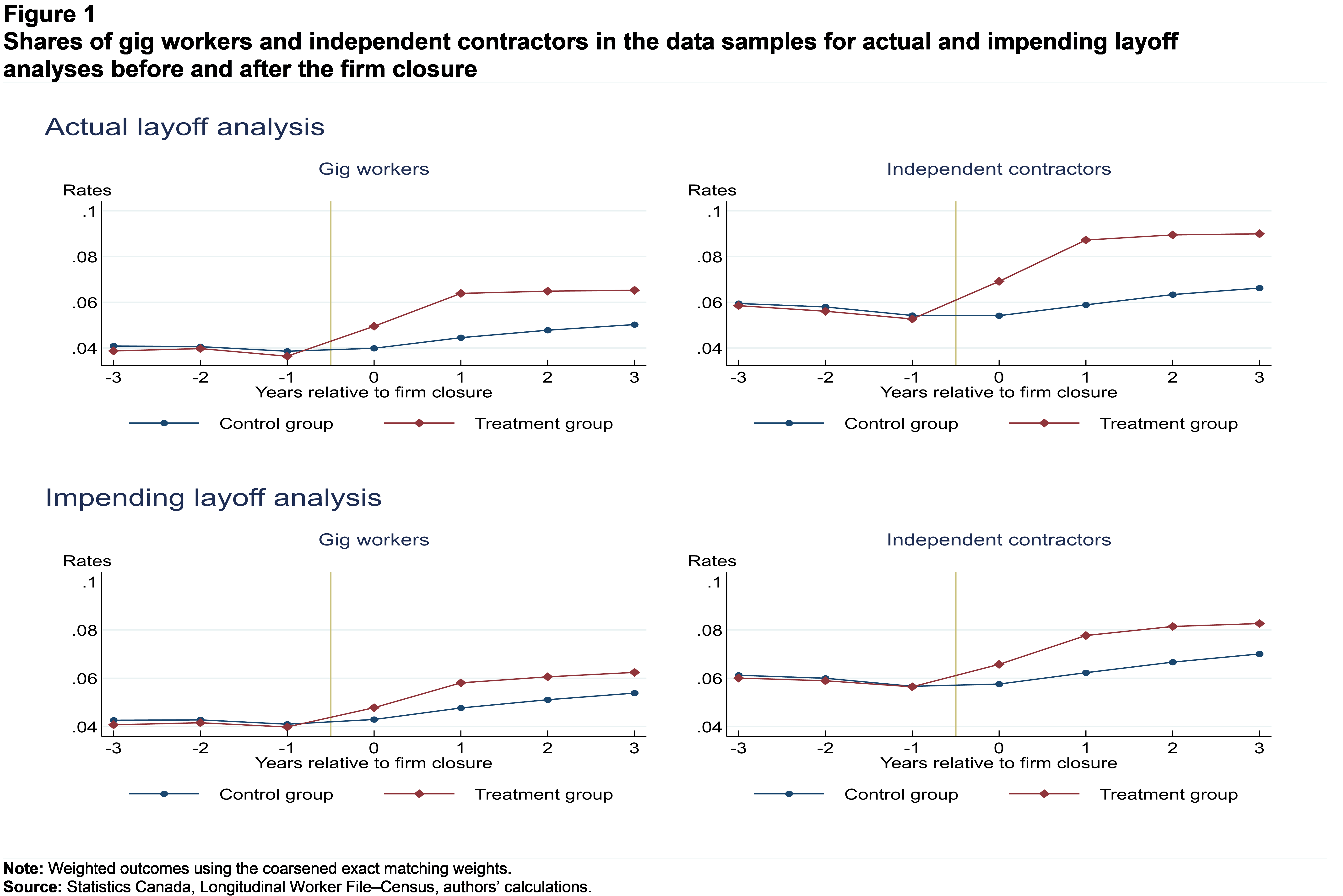
Description for Figure 1
The figure consists of upper and lower horizontal panels, each of which consists of two graphs. In all graphs, the horizontal axes show the year relative to the year of the firm closure () and the vertical axes show the percentages of gig workers or independent contractors among the treatment and control groups in each year. Yearly data points are connected, so each graph shows two lines: one for the treatment group and one for the control group.
The upper panel shows the shares of gig workers (graph on the left) and independent contractors (graph on the right) in the treatment and control groups in the actual layoff sample. The figure on the left shows very similar shares of gig workers in both treatment and control groups in the years before the firm closure, about 4%. The share of gig workers rises sharply in the treatment group to about 6% in the year after the firm closure year, while in the control group, the increase is much weaker, between 4% and 5%. The figure on the right shows similar trends among the treatment and control groups in the analysis of independent contractors, though the percentages are higher: between 5% and 6% before the firm closure, and close to 9% in the treatment group and about 6% in the control group in the year following the year of the firm closure.
The lower panel shows the shares of gig workers (graph on the left) and independent contractors (graph on the right) in the treatment and control groups in the impending layoff sample. The patterns are very similar to those shown in the upper panel graphs.
The linear probability fixed-effects model used to estimate in the matched sample is given by
where is the individual fixed effect absorbing the effects of all the time-invariant unobservables, is a dummy variable corresponding to the year relative to the “base” year and is a dummy variable equal to one if is in the treatment group and zero otherwise. The main coefficients of interest are , which represent the estimated difference in the probability of being a gig worker (independent contractor) between the treatment and control groups in each pre- and post-treatment period and also represent consistent ATT estimates for all post- periods. Consistent estimates of can be obtained from a CEM-weighted regression specified in (2).
5 Results
5.1 Main results
Following the conventions of the literature on job displacement, the estimates of are presented graphically in Figure 2. (The full set of the estimates is available upon request.) The top panel shows for the AL analysis. For both outcomes, and are very small and not statistically significant. This is consistent with the main difference-in-difference assumption of no pre-treatment differences between the treatment group and control group related to the probabilities of being a gig worker or an independent contractor. The estimates of increase sharply in the treatment year and rise further in the first post-treatment year, . In the year following the firm closure, the probability of being a gig worker was 2.1 percentage points higher in the treatment group than in the control group, and the probability of being an independent contractor was 3.0 percentage points higher. To put these differences in percentage terms, the baseline probabilities have to be computed for the control group.Note The 0.021 estimate of in implies that the probability of being a gig worker was 48.6% higher in the treatment group than in the control group. For independent contractors, the 0.030 estimate of translates into the 50.6% treatment–control difference in (Table 2).
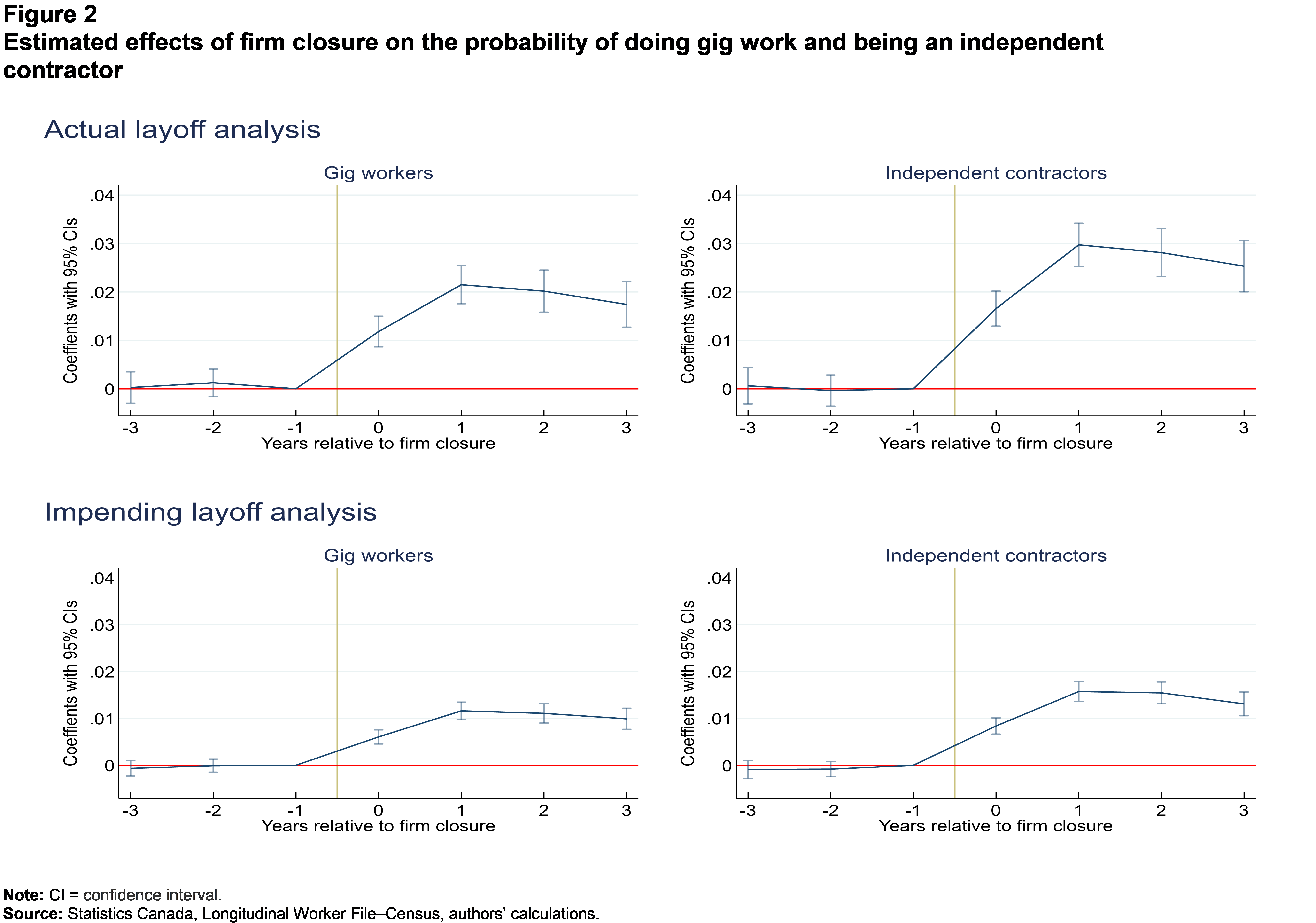
Description for Figure 2
The figure consists of upper and lower horizontal panels, each of which consists of two graphs. The upper panel refers to the actual layoff analysis and the lower panel refers to the impending layoff analysis. In all graphs, the horizontal axes show the year relative to the year of the firm closure and the vertical axes show the estimated effects of firm closure on the probability of being a gig worker or an independent contractor. The line in the graph connects the estimates for each period, with “whiskers” indicating the confidence interval for each estimate.
The graphs indicate various degrees of increase in the probability of being a gig worker or an independent contractor in the treatment group relative to the control group following the firm closure. The estimated post- effects in the actual layoff analysis are roughly double the estimated effects in the impending layoff analysis.
| Actual layoff analysis | Impending layoff analysis | |||
|---|---|---|---|---|
| Gig worker | Independent contractor | Gig worker | Independent contractor | |
| percent | ||||
| x treated | 30.0 | 30.8 | 14.2 | 14.6 |
| x treated | 48.6 | 50.6 | 24.5 | 25.2 |
| x treated | 41.8 | 44.1 | 21.4 | 23.0 |
| x treated | 33.8 | 37.8 | 18.0 | 18.5 |
| Source: Statistics Canada, Longitudinal Worker File-Census, authors' calculations. | ||||
The estimated effects for are only slightly smaller than the estimated effects for : 0.020 for gig workers and 0.028 for independent contractors. The displacement effect gradually fades away, but it was still substantial in : 0.017 for gig workers and 0.025 for independent contractors. In other words, the probability of being a gig worker was 33.8% higher for the treatment group than the control group in , and the probability of being an independent contractor was 37.8% higher.
Figure 2 also shows estimated obtained from the IL analysis (bottom panel). The estimated effects were smaller than in the AL analysis but statistically significant in and in each post- period. In , the estimated effect was 0.012 for gig workers and 0.016 for independent contractors—slightly over half of the estimated effects in the main analysis. This means that the probability of being a gig worker in was 24.5% higher for the treatment group than the control group, and the probability of being an independent contractor was 25.2% higher (Table 2). In , the corresponding effects were 0.010 (18.0%) and 0.013 (18.5%). Compared with the estimates for the AL sample, these results seem to indicate that gig work and independent contracting are strongly related to workers’ ability to find new employment when faced with an impending firm close. This is consistent with the IL treatment group being generally younger, more educated, more likely to be employed in finance and insurance, health care and management and less likely to be employed in agriculture, construction and manufacturing than the AL treatment group (Table 1).Note Those who had remained with the closing firm until the end were substantially more likely to do gig work later than those who had left the firm before the closure, either because their post- earnings were lower than they had been before the firm closure and they needed to supplement their income or because they were unable to find suitable reemployment.
The estimation results shown above are in line with previous findings suggesting that informal work is often a side activity helping wage earners to supplement their income (Hall & Krueger, 2018; Lim et al., 2019). Finding reemployment is likely to be the first priority of displaced workers, but wages and salaries are known to fall after layoffs (Hijzen et al., 2010; Jacobson et al., 1993; Morissette et al., 2013), so it is possible that a fairly large share of displaced workers turn to informal work to supplement their income after they find a new job. It is also possible that, for some individuals, transition to informal work was the main objective of their post-displacement labour market strategy, but having made the transition, they found their income to be insufficient and had to take on a more traditional job. Figure 3 shows that the median earnings (wages and salaries) replacement rate for displaced workers in relative to was 70% in the AL analysis. Not only did displaced workers earn less than the controls in , they also earned considerably less than they had before the layoff.Note
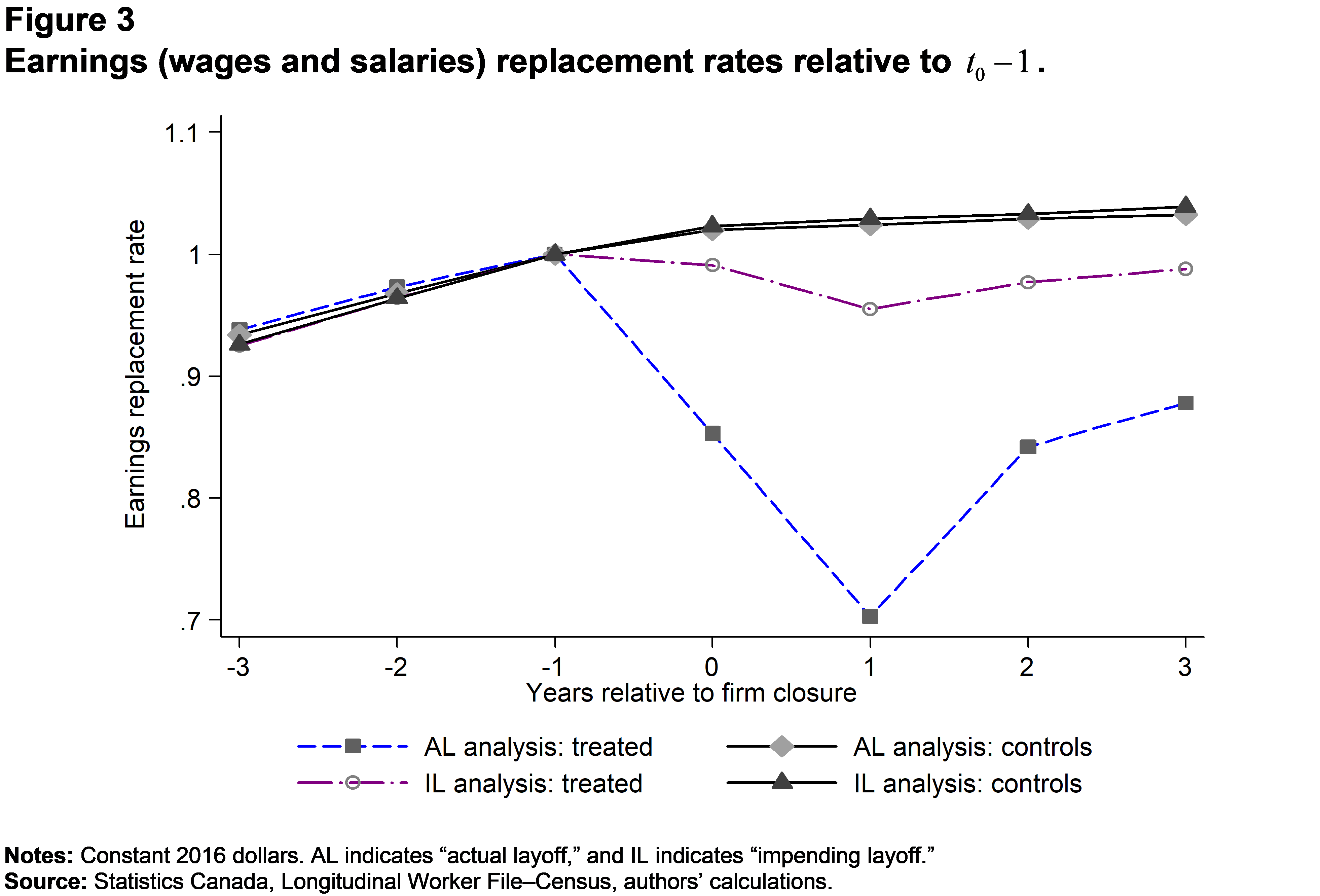
Description for Figure 3
The figure shows earnings (wages and salaries) replacement rates relative to . The horizontal axis shows years relative to , and the vertical axis show the median earnings “replacement rate” or the median ratio of the earnings in each period (numerator) to the earnings in . There are four lines in the graph corresponding to the median ratios for the treatment and control groups in the actual and impending layoff analyses.
All four lines are upward-sloping and almost coincide with each other in all pre- periods. In the years after , the line for the treatment group in the actual layoff analysis takes a deep dive from 1 in to about 0.7 in but increases afterwards to about 0.86 in . The decline for the treatment group in the impending layoff analysis is much smaller (about 0.95 in ). The line for the control groups shows no decline and continues to increase in the post- periods, albeit at a slower pace than before .
Although the motivation for combining informal work with more traditional employment cannot be determined in this study, further insights into the relationship between post-displacement reemployment and participation in informal work were sought by comparing the shares of gig workers and independent contractors among all displaced workers with the shares of gig workers and independent contractors who also earned wages and salaries (T4 earnings) in each period following the displacement in the AL analysis (Table 3). Because all individuals in the sample had to have earnings in and , there was no difference between the percentages of gig workers with and without T4 earnings in those periods. The percentage of displaced workers who were gig workers rose sharply from 3.6% in to 6.4% in and held steady at that level in each of the post- periods (first column). The second column of Table 3 shows that more than two-thirds of gig workers and independent contractors in and about 60% in and —a substantial majority—also earned wages in salaries. The percentages were similar for independent contractors.
| Gig workers | Independent contractors | |||
|---|---|---|---|---|
| All | With T4 | All | With T4 | |
| percent | ||||
| 3.9 | 3.1 | 5.9 | 4.6 | |
| 4.0 | 3.4 | 5.6 | 4.8 | |
| 3.6 | 3.6 | 5.3 | 5.3 | |
| 5.0 | 5.0 | 6.9 | 6.9 | |
| 6.4 | 4.1 | 8.7 | 5.6 | |
| 6.5 | 3.9 | 9.0 | 5.5 | |
| 6.5 | 3.9 | 9.0 | 5.4 | |
| Source: Statistics Canada, Longitudinal Worker File-Census, authors' calculations. | ||||
5.2 How much of the post-treatment gig work is new?
In the analysis above, no restrictions were imposed on participation in gig work or being an independent contractor during the pre- years, so some of those observed in gig work (or as independent contractors) during the post- years were also gig workers (independent contractors) before . It is not immediately clear from the analysis above how displacement and firm closure are related to first-time entry into informal work. To shed light on this and test the robustness of the result above, the sample was restricted to only individuals with no positive outcomes during the three-year period before . For the gig work analysis, this meant that neither treated nor control workers were observed in gig work in any of the three pre- years. Similarly, for the independent contractor analysis, no workers were independent contractors before .Note The new treatment groups were re-matched and the fixed-effects models for each outcome were estimated using new sets of CEM weights.
The results are shown in Figure 4.Note The AL analysis suggests that the probability of being a gig worker in was 2.3 percentage points higher for the treatment group compared with the control group. In relative terms, the probability of being a gig worker was 111.8% higher in the treatment group than in the control group (Table 4). The corresponding effect on the probability of being an independent contractor in was 3.2 percentage points or 126.3%. It appears that the increase in the predicted probability of being a gig worker in reflects primarily new entries in that period, while those who entered gig work before largely continued their involvement in gig work after . The pattern of the IL results is similar to the pattern of the results in the AL analysis: the size of the firm closure effect in each period is roughly half of what it is in the AL analysis. These results confirm lower propensity for taking up informal work among the treatment group that also included individuals who left the closing firm before the actual closure took place compared with the treatment group that included only laid-off workers.
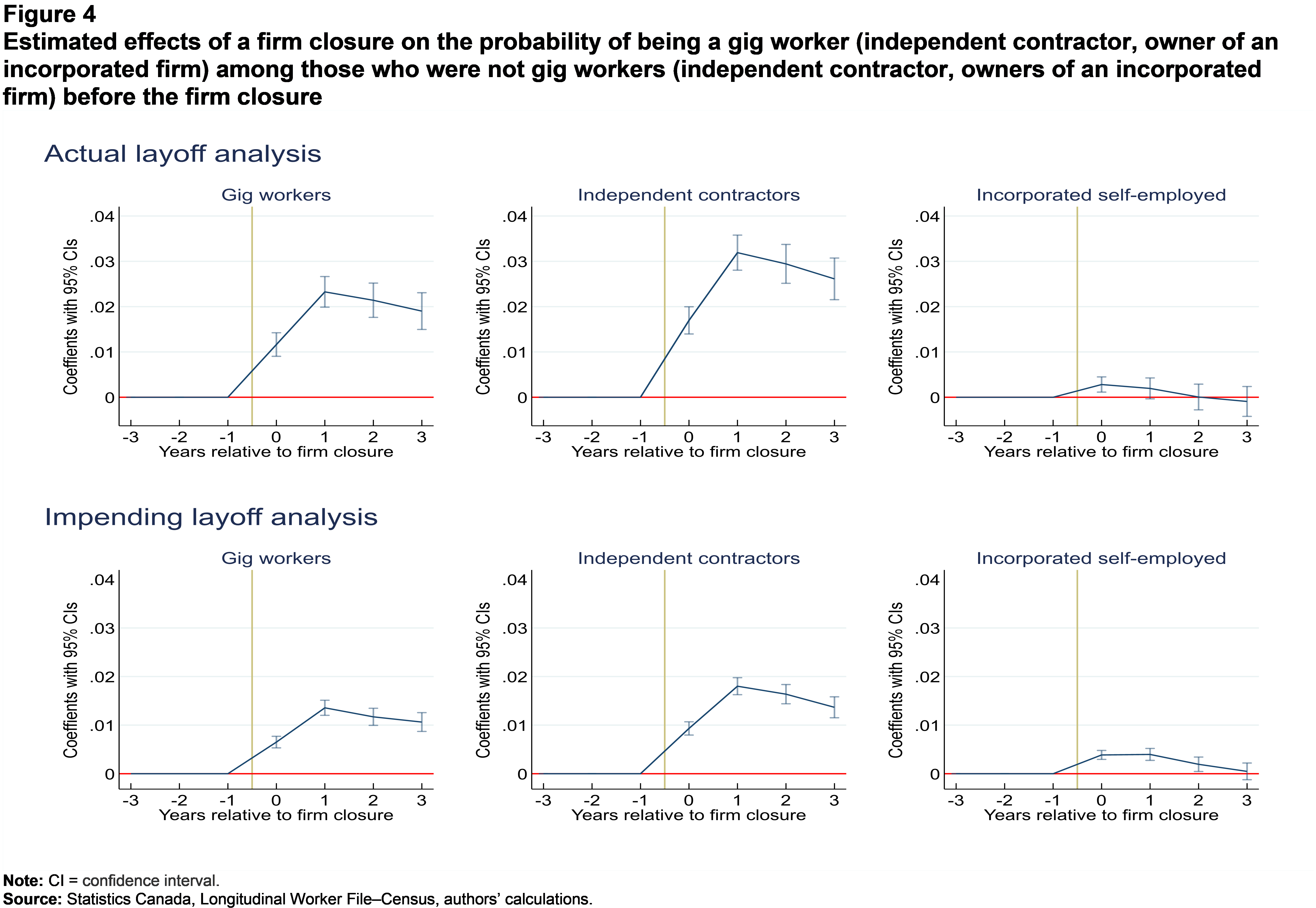
Description for Figure 4
The figure shows estimated effects of a firm closure on the probability of being a gig worker or an independent contractor, or an owner of an incorporated firm, among those who were not gig workers (independent contractor, owners of an incorporated firm) before the firm closure. The figure consists of upper and lower horizontal panels, each of which consists of three graphs: one for the gig work analysis (left), another one for the independent contractor analysis (centre) and the other one for the analysis related to owners of incorporated businesses (right). The upper panel refers to the actual layoff analysis and the lower panel refers to the impending layoff analysis. In all graphs, the horizontal axes show years relative to , and the vertical axes show regression estimates of the effects of the firm closure with “whiskers” indicating confidence intervals.
Similar to Figure 2, the lines connecting period-specific estimates are close to the zero line in all pre- periods in all graphs but show positive and statistically significant effects in the post- periods in the left and centre graphs in both panels. In contrast, the effect of a firm closure on the probability of owning an incorporated business is very small in , and it is not statistically significant in subsequent periods.
| Actual layoff analysis | Impending layoff analysis | |||||
|---|---|---|---|---|---|---|
| Gig worker | Independent contractor | Owner of an incorporated firm | Gig worker | Independent contractor | Owner of an incorporated firm | |
| percent | ||||||
| x treated | 88.7 | 105.5 | 35.7 | 45.6 | 52.9 | 45.3 |
| x treated | 111.8 | 126.3 | 11.6 | 58.7 | 65.0 | 22.8 |
| x treated | 79.0 | 90.1 | 0.2 | 39.2 | 45.9 | 7.5 |
| x treated | 61.5 | 70.2 | -2.9 | 30.7 | 33.1 | 1.5 |
| Source: Statistics Canada, Longitudinal Worker File-Census, authors' calculations. | ||||||
One of the main aspects of informal work is the flexibility of entry and exit from it, since these types of work arrangements require minimal commitment and little investment capital from those who enter them. If the effect of displacement on entry into other forms of self-employment—those that require stronger commitment and larger investment capital—was similar to the estimated effects of displacement on entry into informal work, it would add a great deal of ambiguity to the interpretation of the results above and raise further questions about the relevance of the results specifically to informal work.
As mentioned in Section 4, the data used in this study make it possible to investigate this possibility by estimating the effect of permanent layoff and firm closure on entry into ownership of an incorporated firm and comparing the results with those for entry into informal work. Based on the AL analysis, Figure 4 shows that the impact on entry into incorporated self-employment is much smaller in than for other outcomes (0.003) and virtually non-existent in any post- period. In percentage terms, the probability of entry into incorporated self-employment is 11.6% higher for the treatment group than for the controls in and close to zero for other periods.Note Notably, the estimated effects in the IL analysis for entry into ownership of incorporated firms are somewhat larger than in the main sample, which is the opposite of what was observed for gig work. One possible explanation for this result lies in the distinction between “necessity” and “opportunity” self-employment discussed in Fairlie and Fossen (2020) and the broader differences between the motivations for incorporated and unincorporated self-employment analyzed in Levine and Rubenstein (2017). Entry into incorporated self-employment is likely to be driven more by “opportunity” considerations than entry into informal work, so the link between displacement and entry into ownership of incorporated enterprises is equally weak for those who stay with the closing firms until the end or those who leave in anticipation of the closure.
Previous studies found that much of gig work does not last long. Jeon et al. (2021) reported that just over half of those who enter gig work remain gig workers for at least one year, about 35% remain gig workers for two consecutive years and slightly over one-quarter remain gig workers for three consecutive years. Since much of gig work in post- periods is done in addition to earning wages and salaries, the question is, what was a typical duration of involvement in gig work for displaced workers? Table 5 shows that among displaced workers who entered gig work in , 54.9% were still doing gig work in , 35.6% were still doing gig work in and 28% were still doing gig work in Those who entered into gig work during the displacement year appeared to stay in gig work slightly longer than those who entered during the next year. Among those who entered gig work in , 51.2% continued in and 35.5% in The percentages of those who remain independent contractors were slightly higher in post-entry years than percentages of gig workers.
| Actual layoff sample | Impending layoff sample | |||
|---|---|---|---|---|
| Gig workers | Independent contractors | Gig workers | Independent contractors | |
| percent | ||||
| Enter informal work in (100%) | 100.0 | 100.0 | 100.0 | 100.0 |
| Still in informal work in | 54.9 | 57.6 | 53.3 | 54.9 |
| Still in informal work in | 35.6 | 37.4 | 33.6 | 35.0 |
| Still in informal work in | 28.0 | 28.9 | 24.9 | 26.0 |
| Enter informal work in (100%) | 100.0 | 100.0 | 100.0 | 100.0 |
| Still in informal work in | 51.2 | 54.6 | 51.0 | 54.0 |
| Still in informal work in | 35.5 | 38.6 | 33.9 | 35.8 |
|
Note: Numbers in the table indicate the percentage of original entrants still in informal work in each post-entry period. Source: Statistics Canada, Longitudinal Worker File-Census, authors' calculations. |
||||
5.3 Heterogeneous aspects of entry into informal work: human capital, industry and age
Levine and Rubenstein (2017) argued that there is a fundamental difference in the characteristics and motivations of incorporated and unincorporated business owners: while owners of incorporated businesses are true “entrepreneurs,” this is generally not the case for unincorporated self-employed individuals who often choose self-employment because they have few good employment options. Yet, as mentioned above, entry into gig work is not necessarily motivated by the same considerations and attracts the same individuals as unincorporated self-employment in general. In particular, informal work may attract individuals with higher levels of human capital than unincorporated self-employment more generally, considering that at least some informal work is done online or through online platforms. Abraham and Houseman (2019) found that the percentage of Americans engaged in informal work was the highest among the college-educated, and that college-educated individuals were about 50% more likely to engage in online activities than those with a high school education or less.Note Similarly, Jeon et al. (2021) observed that, although most gig workers did not have a university degree, the prevalence of gig work was higher among university degree holders than among individuals with low levels of education. The question asked in this study is whether the same pattern holds for displaced workers engaged in informal work in the post- periods.
For insights into the relationship between human capital, displacement and entry into gig work, the models in (1) were re-estimated separately for individuals with (a) less than a high school education, (b) a high school diploma, (c) some postsecondary education and (d) a university degree. The salient feature of the AL analysis related to gig work (upper panel in Figure 5) is the contrast between the pattern of the estimated post- effects for displaced workers with less than a high school education and those with a university degree. The effect in was considerably larger for the latter category (0.032), but it diminished in subsequent periods and became small and not statistically significant in . For those with less than a high school education, the estimated effect in was not very large (0.017), but it was larger in (0.022). The same patterns are observed for independent contractors.
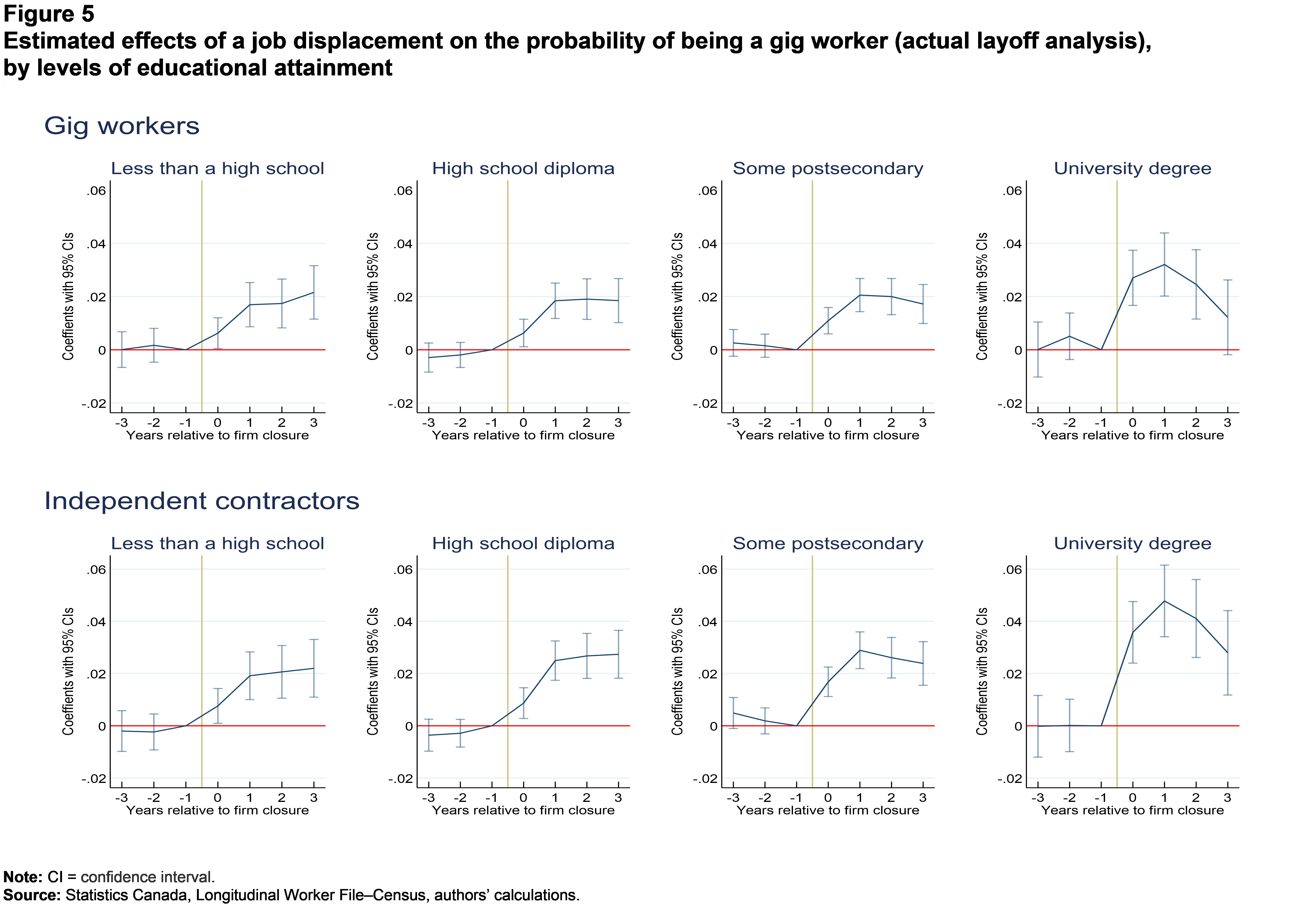
Description for Figure 5
The figure shows estimated effects of a job displacement on the probability of being a gig worker levels of educational attainment. The results are for the actual layoff analysis. The figure consists of upper and lower horizontal panels. Each panel consists of four graphs corresponding to four levels of educational attainment: less than a high school diploma, high school diploma or equivalent, some postsecondary education, and a university degree.
In all graphs, the horizontal axes show years relative to , and the vertical axes show regression estimates of the effects of the firm closure with “whiskers” indicating confidence intervals. The upper panel shows the results for the gig work analysis. The largest increase in the probability of being a gig worker in (close to 0.3) is observed for university degree holders, but the estimate profile is downward sloping after that (just above 1 in ). The increase for the “less than a high school diploma” category is smaller in (about 0.08), but the estimate line is upward sloping so the estimated effect in is higher (about 0.1). The patterns in the lower panel (independent contractors) are similar but the effects are stronger, roughly double of what they are in the gig work analysis.
Part of the difference between the patterns observed for high and low educational categories can probably be explained by the greater flexibility that highly educated workers have over the time and place of their work, and the greater ability of highly educated workers to work autonomously or complete their tasks using online tools (Mas & Pallais, 2020). This flexibility allows highly educated workers to enter informal work more easily when they need extra income, but once they find suitable reemployment, the need for extra income is likely to diminish. Less educated individuals, particularly those working in the service sector or manufacturing, do not have the same flexibility. Mas and Pallais (2020) report that 14% of workers with a high school diploma or less can feasibly complete their jobs from home, compared with 41% for college graduates.
Other heterogeneous aspects of the effects of firm closures on the probability of participating in gig activities have also been considered. The results suggest substantial cross-industry differences in the magnitude and the duration of post- effects. The Canadian economy lost about 500,000 manufacturing jobs from 2000 to the mid-2010s (Morissette, 2020), and workers displaced from manufacturing firms (close to 27% of the treated sample in the AL analysis) were substantially more likely to be engaged in gig work than the control group in all post- periods. The results for retail trade reveal similar patterns, but the number of individuals observed in gig work in other industries was generally too small for the results to be conclusive.Note
Finally, younger workers (25 to 34 years) were notably less likely to engage in gig activities following a firm closure than workers older than 45, and particularly those aged 55 to 59. Possible explanations for this result include the relative scarcity of reemployment opportunities for older workers compared with younger ones and also lesser geographic and occupational mobility often required for reemployment.
6 Conclusions
The main objective of this study was to provide conclusive evidence of the impact of job loss on entry into gig work. Similar to several influential recent studies on gig work, the study identifies gig workers as independent contractors, freelancers, day labourers and on-demand platform workers. Recognizing the conceptual uncertainty surrounding the term “gig worker,” the study also considers an expense-based definition of an “independent contractor.” In addition to gauging direct consequences of involuntary displacement caused by a firm closure, the study uses the “intention-to-treat” framework to account for possible actions taken by workers anticipating an impending closure of the firm that employs them and to gain further insights into the role of (impending) job loss on becoming a gig worker.
The study found that workers displaced by firm closures were about 50% more likely to be gig workers in the year following the displacement year than workers with similar characteristics who did not work in closing firms. The probability of a new entry into gig work among displaced workers was about twice the probability of a new entry among a closely matched control group. However, the study also found that the effect of displacement on the probability of being a gig worker after the displacement is much smaller under the assumptions of the “intention-to-treat” framework, which allows workers to take actions before the firm finally closes its doors.
This is the first study that offers direct evidence of how involuntary job loss and firm closures impact gig work decisions. Research on the impact of job loss on gig work is likely to take greater urgency in the wake of the COVID-19 pandemic, which not only resulted in extensive job losses caused by widespread firm closures in many countries, but also led to fundamental changes in how individuals work and interact. High-quality longitudinal data that would allow researchers to analyze the direct impact of COVID-19 on gig work are not likely to be available for some time. However, in the absence of real-time data, the results of this study provide important and timely clues regarding the magnitude of this impact and how it differs across different categories of workers.
References
Abraham, K., Haltiwanger, J., Sandusky, K., & Spletzer, J. (2018). Measuring the gig economy: Current knowledge and open issues. Cambridge, MA: National Bureau of Economic Research, Working Paper 24950.
Abraham, K., Haltiwanger, J., Sandusky, K., & Spletzer, J. (2019). The rise of the gig economy: fact or fiction? AEA Papers and Proceedings, 109, 357–361.
Abraham, K., & Houseman, S. (2019). Making ends meet: the role of informal work in supplementing Americans’ income. RSF: The Russell Sage Foundation Journal of the Social Sciences, 5(5), 110–131.
Athey, S., & Imbens, G. (2017). The state of applied econometrics: Causality and policy evaluation. Journal of Economic Perspectives, 31(2), 3–32.
Blackwell, M., Iacus, S., King, G., & Porro, G. (2009). cem: Coarsened exact matching in Stata. The Stata Journal, 9(4), 524–546.
Boeri, T., Giupponi, G., Krueger, A., & Machin, S. (2020). Solo self-employment and alternative work arrangements: A cross-country perspective on the changing composition of jobs. Journal of Economic Perspectives, 34(1), 170–195.
Bracha, A., & Burke, M. (2021). How Big is the Gig? The Extensive Margin, The Intensive Margin, and The Hidden Margin. Labour Economics, 69, 101974.
Collins, B., Garin, A., Jackson, E., Koustas, D., & Payne, M. (2020). Has the gig economy replaced traditional jobs over the last two decades? Evidence from tax returns. Unpublished manuscript.
Couch, K., & Placzek, D. (2010). Earnings losses of displaced workers revisited. American Economic Review, 100(1), 572–589.
Detry, M., & Lewis, R. (2014). The intention-to-treat principle: how to assess the true effect of choosing a medical treatment. JAMA, 312(1), 85–86.
Donovan, S., Bradley, D., & Shimabukuru, J. (2016, February). What does the gig economy mean for workers? Congressional Research Service. Retrieved from https://ecommons.cornell.edu/bitstream/handle/1813/79155/CRS_What_does_the_gig_economy_mean.pdf?sequence=1&isAllowed=y.
Evans, D., & Jovanovic, B. (1989). An estimated model of entrepreneurial choice under liquidity constraints. Journal of Political Economy, 97(4), 808–827.
Fairlie, R., & Fossen, F. (2020). Defining opportunity versus necessity entrepreneurship: Two components of business creation. In S. Polachek, & K. Tatsiramos, Change at home, in the labor market, and on the job (Research in Labor Economics), Vol. 48. Emerald Publishing Limited.
Fairlie, R., & Krashinsky, H. (2012). Liquidity constraints, household wealth, and entrepreneurship revisited. Review of Income and Wealth, 58(2), 279–306.
Farber, H. (1999). Alternative and part-time employment arrangements as a response to job loss. Journal of Labor Economics, 17(S4), S142–S169.
Garin, A., Jackson, E., Koustas, D., & McPherson, C. (2020). Is New Platform Work Different from Other Freelancing? AEA Papers and Proceedings, 110, 157–161.
Gupta, S. K. (2011). Intention-to-treat concept: A review. Perspectives in Clinical Research, 2(3), 109–112.
Hall, J., & Krueger, A. (2018). An analysis of the labor market for Uber’s driver-partners in the United States. ILR Review, 71(3), 705–732.
Hijzen, A., Upward, R., & Wright, P. (2010). The income losses of displaced workers. Journal of Human Resources, 45(1), 243–269.
Iacus, S., King, G., & Porro, G. (2011). Multivariate matching methods that are monotonic imbalance bounding. Journal of the American Statistical Association, 106(493), 345–361.
Iacus, S., King, G., & Porro, G. (2012). Causal inference without balance checking: Coarsened exact matching. Political Analysis, 20(1), 1–24.
Iacus, S., King, G., & Porro, G. (2019). A theory of statistical inference for matching methods in causal research. Political Analysis, 27(1), 46–68.
Imai, K., Kim, I. S., & Wang, E. H. (2021). Matching methods for causal inference with time-series cross-sectional data. American Journal of Political Science, 1–19.
Imai, K., King, G., Stuart, E., & others. (2008). Misunderstandings between experimentalists and observationalists about causal inference. Journal of the Royal Statistical Society Series A, 171(2), 481–502.
Imbens, G. (2004). Nonparametric estimation of average treatment effects under exogeneity: A review. Review of Economics and Statistics, 86(1), 4–29.
Imbens, G., & Rubin, D. (2015). Causal inference in statistics, social, and biomedical sciences. Cambridge University Press.
Jackson, E. (2019). Availability of the gig economy and long run supply effects for the unemployed. Stanford University, Stanford, CA. Stanford, CA: Stanford University. Retrieved from https://drive.google.com/file/d/1q1P11aR8oGDy4znTO2GZiNAL-efn33fK/view.
Jackson, E., Looney, A., & Ramnath, S. (2017). The rise of alternative work arrangements: Evidence and implications for tax filing and benefit coverage. Technical, Office of Tax Analysis Working Paper, 114.
Jacobson, L. S., LaLonde, R. J., & Sullivan, D. G. (1993). Earnings losses of displaced workers. American Economic Review, 685–709.
Jeon, S.-H., Liu, H., & Ostrovsky, Y. (2021). Measuring the gig economy in Canada using administrative data. Canadian Journal of Economics, 54(4).
Katz, L., & Krueger, A. (2017). The role of unemployment in the rise in alternative work arrangements. American Economic Review, 107(5), 388–392.
Kostyshyna, O., & Luu, C. (2019). The Size and Characteristics of Informal (“Gig”) Work in Canada. Bank of Canada. Ottawa: Bank of Canada.
Koustas, D. (2019). What do big data tell us about why people take gig economy jobs? AEA Papers and Proceedings, 109, 367–371.
Koustas, D. (2020). Insights from New Tax-Based Measures of Gig Work in the United States. München: ifo Institut-Leibniz-Institut für Wirtschaftsforschung an der~…, 21, pp. 5--9.
Krashinsky, H. (2004). Self-employment for less-educated men. Technical, Mimeo, University of Toronto.
Levine, R., & Rubinstein, Y. (2017). Smart and illicit: who becomes an entrepreneur and do they earn more? The Quarterly Journal of Economics, 132(2), 963–1018.
Lim, K., Miller, A., Risch, M., & Wilking, E. (2019). Independent contractors in the US: New trends from 15 years of administrative tax data. Internal Revenue Services (IRS). Internal Revenue Services, no. 45. Retrieved from https://www.irs.gov/pub/irs-soi/19rpindcontractorinus.pdf.
Mas, A., & Pallais, A. (2020). Alternative work arrangements. Annual Review of Economics, 12, 631–658.
Morissette, R. (2020). The Impact of the Manufacturing Decline on Local Labour Markets in Canada. Ottawa: ASB Research Paper Series, Statistics Canada.
Morissette, R., Qiu, H., & & Chan, P. C. (2013). The risk and cost of job loss in Canada, 1978–2008. Canadian Journal of Economics, 46(4), 1480–1509.
Simoes, N., Crespo, N., & Moreira, S. (2016). Individual determinants of self-employment entry: What do we really know? Journal of Economic Surveys, 30(4), 783–806.
Statistics Canada. (2019). Sampling and weighting for the long form. Retrieved from Guide to the Census of Population, 2016: https://www12.statcan.gc.ca/census-recensement/2016/ref/98-304/chap9-eng.cfm.
Stevens, A. H. (1997). Persistent Effects of Job Displacement: The Importance of Multiple Job Losses. Journal of Labor Economics, 15, 165–188.
Stuart, E. (2010). Matching Methods for Causal Inference: A Review and a Look Forward. Statistical Science, 1–21.
Von Greiff, J. (2009). Displacement and self-employment entry. Labour Economics, 16(5), 556–565.
Wooldridge, J. (2002). Econometric analysis of cross section and panel data. MIT Press.
- Date modified: