
Correction Notice
A correction has been made to Table 2 titled: Descriptive statistics by birth cohort. The Gini coefficient for parental after-tax income in 1963 has been corrected.
Acknowledgement
The Social Analysis and Modelling Division at Statistics Canada engaged in a collaborative initiative with Dr. Marie Connolly and Dr. Catherine Haeck to augment and update Statistics Canada’s Intergenerational Income Database (IID). Supported by funding obtained by Drs. Connolly and Haeck, Statistics Canada added three cohorts of teens and parents to the IID and extended the reference period covered by the file. Drs. Connolly and Haeck also worked closely with Statistics Canada staff to validate and document the updated file. The data file, which is accessible to researchers through the Canadian Research Data Centre Network, allows intergenerational comparisons of income mobility in Canada to be drawn across a wider range of birth cohorts, over a longer period of time, than was previously possible. Statistics Canada is pleased to publish Drs. Connolly and Haeck’s research on this important topic and thanks them for their collaboration on this initiative.
Abstract
While cross-sectional increases in inequality are a cause for concern, the study of the intergenerational transmission of income is perhaps more relevant for understanding trends in inequality over time. How is social status reproduced from one generation to the next? Recent work has highlighted the relationship—if not causal, then correlational—between inequality and measures of social mobility in a cross-country setting. This relationship is dubbed the Great Gatsby Curve (Corak 2013): regions with higher inequality in childhood tend to have lower intergenerational income mobility between the child and their parents.
In this paper, administrative Canadian tax data are exploited to compute measures of intergenerational income mobility at the national, provincial and territorial levels. This work provides detailed descriptive evidence on trends in social mobility. Results show that mobility has steadily declined over time and that there has been an increase in the inequality of the parental income distribution, as measured by the Gini coefficient. Therefore, Canada and all its provinces have been “going up” the Great Gatsby Curve. The cross-sectional, cross-country relationship observed in the literature thus also holds within a country over time, lending credence to the more causal than correlational nature of the relationship, though causality is not formally tested here.
JEL: J62, D63
Keywords: Canada, Great Gatsby Curve, income inequality, intergenerational transmission, social mobility
Executive summary
While cross-sectional increases in inequality are a cause for concern, the study of the intergenerational transmission of income is perhaps more relevant for understanding trends in inequality over time. How is social status reproduced from one generation to the next? Recent work has highlighted the relationship—if not causal, then correlational—between inequality and measures of social mobility in a cross-country setting. This relationship is dubbed the Great Gatsby Curve (Corak 2013): regions with higher inequality in childhood tend to have lower intergenerational income mobility between the child and their parents.
Results show that mobility has steadily declined over time and that there has been an increase in the inequality of the parental income distribution, as measured by the Gini coefficient. Therefore, Canada and all its provinces have been “going up” the Great Gatsby Curve. The cross-sectional, cross-country relationship observed in the literature thus also holds within a country over time, lending credence to the more causal than correlational nature of the relationship, though causality is not formally tested here.
The focus is on rank mobility, and findings show that the correlation between a child’s income rank, as an adult, and their parents’ income rank has been trending up, increasing from 0.189 among the 1963-to-1966 birth cohort to 0.234 among the 1982-to-1985 cohort. There also appears to be substantial nonlinearity in the rank mobility equation. The rank-rank slopes are higher, thus indicating lower mobility, for children from lower parental income ranks. Moreover, the average child ranks for the more recent cohorts are lower than those of the first cohort for a substantial part of the bottom of the parental income distribution: even children whose parents are at the 30th to 35th percentiles have lower average ranks for the 1982-to-1985 cohort than for the 1963-to-1966 cohort.
Rank mobility is also described at the provincial and territorial levels. While there has been a deterioration of mobility in every single province, there are still large variations in rank-rank slopes across regions in the most recent cohort, and the within-province variations over time have different magnitudes. Some places, notably the Atlantic provinces, have among the lowest rank-rank slopes, meaning the most equal opportunities for children, along with the smallest increases in slopes. Manitoba generally displays the lowest intergenerational mobility among the 10 provinces, and it is in Saskatchewan that the deterioration of equality of opportunities has been the worst. A look at quintile transition matrices reveals much the same story of declining mobility: children born in families with a total family income in the bottom 20% of the income distribution have become less likely to exit the bottom quintile themselves and less likely to transition into the middle class.
1 Introduction
In Canada, as in most other parts of the world, income inequality is on the rise (Heisz 2016). For example, in Canada, the national income share of the top 1% increased from 8.9% to 13.6% between 1980 and 2010 when measured using repeated cross-sectional estimates. In the United States, the top 1% share went from 10.7% to 19.8% over the same time period; in the United Kingdom, the increase was from 5.9% to 12.5% (Alvaredo et al. 2018). A complementary perspective on income inequality can be obtained by assessing it in terms of intergenerational income mobility—that is, the extent to which one’s place in the income distribution in adulthood is correlated with the location of one’s parents at an earlier point in time. In short, how likely is it that children from the bottom or top of the income distribution themselves end up at the bottom or top of the distribution later in life? In this paper, three measures of intergenerational income mobility are discussed and applied to Canadian data. Five cohorts of Canadians, born between 1963 and 1985, are observed as teens living with their parents and again as adults in their late 20s and early 30s. The three measures of intergenerational income mobility all indicate that the relationship between parents’ and children’s locations in the income distribution became stronger across the five cohorts. For example, transition matrices show that the probability that a child from the bottom 20% of the parental income distribution remained in the bottom quintile increased from 27.1% to 32.6% from the earliest to the most recent of the five birth cohorts. Such patterns are observed at the national and the provincial and territorial levels.
In the international literature, countries are plotted not only in terms of their rate of intergenerational income mobility but also in terms of their degree of income inequality. Recent work has highlighted the relationship—if not causal, then correlational—between intergenerational income mobility and income inequality in a cross-country setting (Corak 2006; Blanden 2013). This relationship is dubbed the Great Gatsby Curve (Corak 2013): countries with higher inequality in childhood tend to have lower intergenerational income mobility between the child and their parents. Results from this analysis show that in addition to a decline in intergenerational income mobility, there has also been an increase in the inequality of parental income across the five cohorts, as measured by the Gini coefficient, at both the national and the provincial levels. This suggests that Canada and the provinces have been “going up” the Great Gatsby Curve.
The remainder of the paper is structured as follows. Section 2 presents information on the data source and methods used for the analysis. Findings are presented in Section 3. The section begins with results on intergenerational mobility at the national level measured using rank mobility and intergenerational elasticity, disaggregated by gender of the child. Nonlinearity in rank mobility is subsequently discussed. Next, rank mobility at the provincial and territorial levels is investigated, followed by trends in income transition matrices. The final subsection locates successive birth cohorts on the Great Gatsby Curve for Canada, linking rank mobility to parental income inequality. Conclusions are presented in Section 4.
2 Data and measures
2.1 Data
Until recently, it was not possible to compare intergenerational income mobility across birth cohorts in Canada because of a lack of suitable data. This changed with the addition of new birth cohorts to Statistics Canada’s Intergenerational Income Database (IID). This database, first developed in the mid-1990s (see Corak and Heisz 1999), contains longitudinal administrative tax files of successive cohorts of children and their parents in Canada. The original IID cohorts covered children born between 1963 and 1970, inclusively, observing them as teens in 1982, 1984 and 1986. More recent cohorts covering most birth years between 1972 and 1985 have been added to the IID.Note
In this paper, all available birth cohorts in the IID are exploited to compute measures of intergenerational income mobility and look at trends at the national and provincial/territorial levels. The sample is split into five successive birth cohorts. Each cohort is identified using the first fiscal year in which the link between the parents and the child is attempted. For example, the 1982 cohort includes children born between 1963 and 1966, who were matched to their parents in 1982, when they were 16 to 19 years old. If the match could not be established in 1982, the match was attempted again over the next four years. To avoid overlapping birth years across different cohorts, the 1984 IID cohort was divided in two, with the older half pooled with the 1982 IID cohort and the younger half pooled with the 1986 IID cohort. Duplicates were removed. Table 1 gives the birth years and number of observations per cohort as defined for this paper. There are over 1 million children per birth cohort, for a total of close to 6 million child–parent pairs.
| IID cohort | Birth years | IID count | IID weighted count |
|---|---|---|---|
| 1982 and 1984 | 1963 to 1966 | 1,219,470 | 1,566,240 |
| 1984 and 1986 | 1967 to 1970 | 1,158,900 | 1,555,280 |
| 1991 | 1972 to 1975 | 1,095,160 | 1,474,140 |
| 1996 | 1977 to 1980 | 1,166,440 | 1,557,800 |
| 2001 | 1982 to 1985 | 1,349,190 | 1,633,270 |
|
Note: IID: Intergenerational Income Database. Source: Authors’ calculations based on Statistics Canada’s Intergenerational Income Database. |
|||
In the IID, tax files are available annually starting in 1978 for the 1982, 1984 and 1986 IID cohorts and starting in 1981 for the more recent cohorts. The last available year of tax data for all cohorts was 2014 at the time of writing. Income measures are available for individuals in the family, including both parents, if present; the child; and, if present, the spouse of the child in adulthood. The analysis is based on total income from all sources, as defined by the Canada Revenue Agency. This includes earnings, interest and investment income, self-employment net income, taxable capital gains or losses and benefits from public programs and transfers. In the main analysis, pre-tax total income is used, with robustness checks done using after-tax income.
Parental income is defined as the average annual parental income when the child was aged 15 to 19 years, including both parents, if present.Note Taking a five-year average reduces biases resulting from transitory shocks to income (Chen, Ostrovsky and Piraino 2017). A five-year window during the late teenage years reflects the resources available to the child during the transition years between secondary and postsecondary school or between schooling and the labour market. These ages are also used because they are the closest to the year in which the family link was created in the tax files. Because biological links are not identified in the IID and because only the adults identified as the child’s parents at the moment of the link can be tracked in fiscal data, calculating family income prior to the teenage years (e.g., early childhood) would be incorrect for children whose parents have separated or divorced prior to age 15. Another reason to use parental income when the child is 15 to 19 years old is that since the tax files start in 1978, data on parental income during early childhood are not available for the first birth cohorts, restricting comparability across cohorts.
Comparability across cohorts becomes an important issue when deciding how to compute the measures of the child’s income in adulthood. If five-year averages are used for child income, as is done for parents, then the oldest age at which individuals in the last cohort can be observed is 25 to 29 years.Note This age band is comparable to Chetty et al.’s (2014a) main analysis (ages 29 to 32) and sensitivity checks (ages 26 to 29). To study trends over the longest period possible using the IID, five-year averages from ages 25 to 29 are used in the main analysis. Child income averages are also computed for the ages of 30 to 34 and 35 to 39. The first four of the five cohorts are used when child income is measured at ages 30 to 34, and the first three cohorts are used when child income is measured at ages 35 to 39. Note that whenever a parent or child is not found in the tax files for a given year, an income of $0 is imputed for that year. The sample is then restricted to children who are observed at least once over the five-year period and to parents and children who have an average income of at least $500. This treatment is consistent with Corak’s (2020) sample selection. Child individual income is used for most of the analysis, with robustness checks done using child family income. All dollar figures are converted to 2016 Canadian dollars using the all-items Consumer Price Index Table No. 18-10-0005-01 (formerly CANSIM Table 326‑0021).
Once the five-year averages are computed for both child and parental income, percentile ranks are computed using the national distribution for most of the analysis and the provincial/territorial distribution for some complementary analysis. The province or territory of residence is fixed at the time of the link between the child and the parents, i.e., when the child is aged 16 to 19. This means that if a child moves out of a province or territory by the time their income is measured, that child is still assigned to the place where they grew up, as was done by Chetty et al. (2014a); Corak (2020); and Connolly, Corak and Haeck (2019). The effects of geographical mobility on income mobility are left for further studies.
Table 2 presents descriptive statistics for each birth cohort. The top panel provides information on parents. Their average income increased over time, from $78,800 among the parents of the 1963 cohort of children to $89,200 among the parents of the 1982 cohort. The standard deviations around these averages increased, as did the Gini coefficients—a measure of inequality—estimated using both before- and after-tax income.
The number of parents linked to a child depends on who filed a tax return the year of the parent-child match. If only one parent filed a tax return, then only that parent is observed in the IID. For the 1963 birth cohort, the proportion of children for whom only one parent filed taxes was 30.8%, while for the 1982 birth cohort it was 21.8%. This does not necessarily reflect a change in family composition (i.e., a decrease in lone-parent families), as two-parent families with only one taxfiling spouse are included in the figures. The rise in women’s labour force participation and the increase in dual-earner families (Statistics Canada 2016) no doubt account for much of the decline observed. This shift is not problematic for this analysis. Parental income reflects resources available in the child’s family, with diminished capacity in this respect reflected in a single parent filing taxes, whether because only one parent is present or because only one parent is employed.
| Birth cohort | |||||
|---|---|---|---|---|---|
| 1963 | 1967 | 1972 | 1977 | 1982 | |
| dollars | |||||
| Average parental income (before tax) | 78,800 | 77,700 | 82,100 | 81,200 | 89,200 |
| Standard deviation | 84,300 | 82,800 | 91,800 | 104,200 | 167,300 |
| coefficient | |||||
| Gini coefficient, parental before-tax income | 36.36 | 37.77 | 39.27 | 41.18 | 44.37 |
| Gini coefficient, parental after-tax income | 34.08 | 34.70 | 36.04 | 37.46 | 40.53 |
| percentage | |||||
| Percentage in one-parent taxfiler household | 30.8 | 29.6 | 24.8 | 23.1 | 21.8 |
| Average child income | dollars | ||||
| Ages 25 to 29 | 34,100 | 32,000 | 34,100 | 35,300 | 36,700 |
| Standard deviation | 23,100 | 24,200 | 27,800 | 27,000 | 30,100 |
| Ages 30 to 34 | 42,100 | 43,600 | 46,100 | 47,700 | Note ...: not applicable |
| Standard deviation | 44,300 | 130,600 | 44,800 | 41,600 | Note ...: not applicable |
| Ages 35 to 39 | 51,500 | 53,600 | 56,500 | Note ...: not applicable | Note ...: not applicable |
| Standard deviation | 73,400 | 77,600 | 63,500 | Note ...: not applicable | Note ...: not applicable |
| coefficient | |||||
| Gini coefficient, child before-tax income | |||||
| Ages 25 to 29 | 33.77 | 35.51 | 35.64 | 36.10 | 38.13 |
| Ages 30 to 34 | 38.52 | 39.87 | 39.26 | 39.03 | Note ...: not applicable |
| Ages 35 to 39 | 42.41 | 43.25 | 42.04 | Note ...: not applicable | Note ...: not applicable |
| Gini coefficient, child after-tax income | |||||
| Ages 25 to 29 | 31.18 | 32.73 | 33.11 | 33.50 | 35.24 |
| Ages 30 to 34 | 35.31 | 36.78 | 36.24 | 36.14 | Note ...: not applicable |
| Ages 35 to 39 | 38.89 | 39.80 | 38.69 | Note ...: not applicable | Note ...: not applicable |
| percentage | |||||
| Percentage female (ages 25 to 29) | 49.02 | 48.71 | 48.86 | 48.95 | 49.10 |
| Percentage single, children | |||||
| Ages 25 to 29 | 51.12 | 49.11 | 52.47 | 55.85 | 57.87 |
| Ages 30 to 34 | 30.76 | 31.08 | 32.03 | 35.03 | Note ...: not applicable |
| Ages 35 to 39 | 24.65 | 25.19 | 26.44 | Note ...: not applicable | Note ...: not applicable |
| number | |||||
| Weighted sample size excluding parents with income under $500 and children missing all years or with five-year average total income under $500 | |||||
| Ages 25 to 29 | 1,469,010 | 1,437,190 | 1,357,900 | 1,442,150 | 1,501,800 |
| Ages 30 to 34 | 1,421,820 | 1,386,020 | 1,321,720 | 1,408,010 | Note ...: not applicable |
| Ages 35 to 39 | 1,393,430 | 1,364,920 | 1,301,780 | Note ...: not applicable | Note ...: not applicable |
| percentage | |||||
| Sample selection, parents | |||||
| Percentage missing at least one year during the five-year window | 7.48 | 8.08 | 10.91 | 9.30 | 10.97 |
| Percentage with income under $500 | 1.83 | 2.20 | 1.85 | 1.71 | 2.15 |
| Sample selection, children | |||||
| Percentage missing from all tax files | |||||
| Ages 25 to 29 | 2.92 | 3.81 | 4.45 | 4.31 | 4.44 |
| Ages 30 to 34 | 4.98 | 6.41 | 6.85 | 6.51 | Note ...: not applicable |
| Ages 35 to 39 | 6.80 | 8.02 | 8.31 | Note ...: not applicable | Note ...: not applicable |
| Percentage missing at least one year during the five-year window | |||||
| Ages 25 to 29 | 19.91 | 23.99 | 24.54 | 24.53 | 24.73 |
| Ages 30 to 34 | 22.53 | 24.79 | 24.86 | 24.10 | Note ...: not applicable |
| Ages 35 to 39 | 23.00 | 25.24 | 24.74 | Note ...: not applicable | Note ...: not applicable |
| Percentage with income under $500, children | |||||
| Ages 25 to 29 | 1.50 | 1.80 | 1.90 | 1.70 | 1.80 |
| Ages 30 to 34 | 2.60 | 2.70 | 2.10 | 1.80 | Note ...: not applicable |
| Ages 35 to 39 | 2.70 | 2.50 | 2.10 | Note ...: not applicable | Note ...: not applicable |
|
... not applicable Source: Authors’ calculations based on Statistics Canada’s Intergenerational Income Database. |
|||||
The second panel of Table 2 presents information pertaining to the (adult) children. Average income at ages 35 to 39 increased across the three oldest birth cohorts, from $51,500 to $56,500. Average income at ages 30 to 34 increased similarly across the four oldest cohorts, as it did at ages 25 to 29 across the four most recent cohorts. Gini coefficients across the cohorts increased, particularly when measured at ages 25 to 29. Gini coefficients observed at ages 30 to 34 and 35 to 39 increased across the two earliest cohorts, but have declined since then.
The bottom two panels investigate the sample selection. At most, 2.2% of parents and 2.7% of children are excluded because their total income was under $500. The fraction of children who are completely missing from the tax data over the relevant five-year interval increased with the age of the child, going from 3% to 4% at ages 25 to 29, to 5% to 7% at ages 30 to 34, to 7% to 8% at ages 35 to 39. The death rate is still very low at those ages, so the attrition most likely reflects outmigration. A nontrivial proportion of both parents and children have at least one year of tax files missing: up to 11% for the parents and up to 25% for the children. In robustness analyses, the sample is further restricted to parents and children observed in all five years. Results do not change using this alternative specification.
2.2 Measures of intergenerational income mobility
Several measures are available to estimate intergenerational income mobility. The intergenerational elasticity (IGE) of income has been widely used in the literature as a measure of mobility (or lack thereof), including in studies based on early IID cohorts in Canada such as those by Corak and Heisz (1999) and Chen, Ostrovsky and Piraino (2017). The IGE of income is typically computed by estimating a linear model where the natural logarithm of child income is explained by the natural logarithm of parental income. However, because of the use of logs, as Dahl and DeLeire (2008), Chetty et al. (2014a) and Connolly, Corak and Haeck (2019) have noted, IGE estimates are sensitive to the treatment of very small values of income. An alternative approach is rank mobility. Rank mobility is defined in much the same fashion as the IGE, except that child income and parental income are measured as percentile ranks in their respective income distribution. Rank mobility has proven to be much more robust to the treatment of low incomes and to different model specifications and is therefore the preferred method used in this analysis. It is estimated using the following model in Equation (1):
where is the income rank of child —the generation—in province or territory is the income rank of their parent or parents—the generation—and is a random term. The slope from Equation (1), can be interpreted as a measure of intergenerational mobility: the higher the the more parental income rank explains child income rank and the less mobility there is. Equation (1) is estimated at both the national and the provincial or territorial levels, where geographical location is fixed during teenage years. The ranks can be computed from the national distribution or the provincial/territorial distribution, and estimates using both types of ranks will be presented. In addition to rank mobility, intergenerational elasticities of income are also presented, estimated using Equation (2) below:
where is the total income of child from province or territory , is their parents’ income and is a random term. The slope of this model, is the IGE of income.
Finally, a third mobility measure that can be computed is the transition matrix. In an income quintile transition matrix, each column refers to a quintile of the parental income distribution and each row to a quintile of the child income distribution. Each cell is a conditional probability. Conditional probabilities are denoted as the probability of moving from origin (parental income quintile) to destination (child income quintile), or Pr(child income quintile |parental income quintile ). As with Corak (2020) and Connolly, Corak and Haeck (2019), the focus is on a few key points of the transition matrix: and The intergenerational cycle of poverty, captures the probability for a child raised in the bottom quintile of the family income distribution to remain in the bottom quintile as an adult. The rags-to-riches movement, is the probability of moving from the bottom to the top income quintile. Finally, measures the probability of moving from the bottom income quintile to the middle three quintiles.
Research in the United States has shown that different conclusions regarding trends in intergenerational income mobility may be reached depending on the data source and methods used. Chetty et al. (2014b) used tax data and found that the rank-rank relationship did not change in the United States between the 1971 and 1982 birth cohorts. Davis and Mazumder (2017) used the National Longitudinal Surveys and found declines in intergenerational mobility between cohorts born in 1942 to 1953 and 1957 to 1964 in both the rank-rank relationship and the IGE of income.
3 Results
This section will go through the results of the analysis, starting with trends in mobility at the national level. For ease of presenting analytical results, birth cohorts are referred to by the first birth year of the cohort (e.g., the 1963 birth cohort designates the 1963-to-1966 birth cohort).
3.1 Mobility at the national level
Table 3 shows the estimated rank-rank slopes from Equation (1), by birth cohort and age at which child income is observed, for sons and daughters combined and separately. The IGE estimates from Equation (2) are also shown. A higher rank-rank slope or a higher IGE means that parental income has a higher explanatory power on child income and, therefore, mobility is lower.
| Birth cohort | |||||
|---|---|---|---|---|---|
| 1963 | 1967 | 1972 | 1977 | 1982 | |
| coefficient | |||||
| Rank-rank | |||||
| Ages 25 to 29 | 0.189 | 0.188 | 0.216 | 0.215 | 0.234 |
| Ages 30 to 34 | 0.201 | 0.214 | 0.232 | 0.235 | Note ...: not applicable |
| Ages 35 to 39 | 0.201 | 0.214 | 0.230 | Note ...: not applicable | Note ...: not applicable |
| Rank-rank for sons | |||||
| Ages 25 to 29 | 0.188 | 0.187 | 0.214 | 0.219 | 0.233 |
| Ages 30 to 34 | 0.227 | 0.237 | 0.252 | 0.253 | Note ...: not applicable |
| Ages 35 to 39 | 0.238 | 0.247 | 0.257 | Note ...: not applicable | Note ...: not applicable |
| Rank-rank for daughters | |||||
| Ages 25 to 29 | 0.204 | 0.200 | 0.228 | 0.216 | 0.238 |
| Ages 30 to 34 | 0.193 | 0.205 | 0.223 | 0.224 | Note ...: not applicable |
| Ages 35 to 39 | 0.182 | 0.194 | 0.214 | Note ...: not applicable | Note ...: not applicable |
| IGE of income | |||||
| Ages 25 to 29 | 0.153 | 0.154 | 0.199 | 0.210 | 0.224 |
| Ages 30 to 34 | 0.171 | 0.184 | 0.223 | 0.239 | Note ...: not applicable |
| Ages 35 to 39 | 0.180 | 0.192 | 0.232 | Note ...: not applicable | Note ...: not applicable |
| IGE of income for sons | |||||
| Ages 25 to 29 | 0.154 | 0.157 | 0.200 | 0.215 | 0.223 |
| Ages 30 to 34 | 0.192 | 0.202 | 0.238 | 0.251 | Note ...: not applicable |
| Ages 35 to 39 | 0.214 | 0.221 | 0.255 | Note ...: not applicable | Note ...: not applicable |
| IGE of income for daughters | |||||
| Ages 25 to 29 | 0.165 | 0.160 | 0.206 | 0.210 | 0.227 |
| Ages 30 to 34 | 0.166 | 0.178 | 0.219 | 0.234 | Note ...: not applicable |
| Ages 35 to 39 | 0.161 | 0.174 | 0.219 | Note ...: not applicable | Note ...: not applicable |
| ... not applicable Note: IGE: Intergenerational elasticity. Source: Authors’ calculations based on Statistics Canada’s Intergenerational Income Database. |
|||||
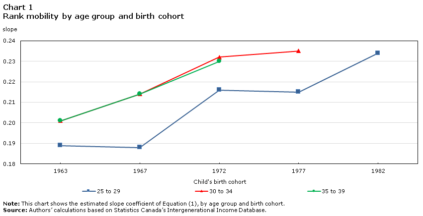
A clear pattern toward decreasing intergenerational mobility can be observed from the earliest to the latest birth cohorts, with the rank-rank slope increasing steadily across them. When measured at ages 25 to 29, the rank-rank slope increased from 0.189 to 0.234 from the 1963 to the 1982 cohort—a 24% increase. This trend is evident for both sons (increasing from 0.188 to 0.233) and daughters (increasing from 0.204 to 0.238). IGE also increased across birth cohorts, again indicating less intergenerational mobility. Among sons and daughters combined, the IGE increased from 0.153 to 0.224 from the 1963 to the 1982 cohort, with increases observed for both genders. The upward trend is also observed at older ages, even if the point estimates tend to be slightly larger the older the child. Chart 1 shows the rank-rank slope at different ages among sons and daughters combined, using the data points from Table 1.
Data table for Chart 1
| Child's birth cohort | 25 to 29 | 30 to 34 | 35 to 39 |
|---|---|---|---|
| slope | |||
| 1963 | 0.19 | 0.20 | 0.20 |
| 1967 | 0.19 | 0.21 | 0.21 |
| 1972 | 0.22 | 0.23 | 0.23 |
| 1977 | 0.22 | 0.24 | Note ...: not applicable |
| 1982 | 0.23 | Note ...: not applicable | Note ...: not applicable |
|
... not applicable Note: This chart shows the estimated slope coefficient of Equation (1), by age group and birth cohort. Source: Authors’ calculations based on Statistics Canada’s Intergenerational Income Database. |
|||
3.2 Nonlinearity in rank mobility
Given the increasing correlation between parent and child locations in the income distribution, a further question is whether this trend is being driven by changes at the bottom, in the middle or at the top of the parental income distribution. Among which segments of the distribution is opportunity for mobility declining most?
To investigate, locally weighted nonparametric smoothed scatter plots were estimated for each birth cohort and are presented in Chart 2. The curves show the average rank in the income distribution achieved by children from each percentile of the parental income distribution. The curves are not linear, with the slope steeper at the lower end and, to a lesser degree, the higher end of the parental income distribution. Each curve represents a birth cohort. These turn out to be approximately stacked in order of birth years. At the bottom of the distribution, earlier cohorts have higher mean child ranks than later cohorts—meaning that, on average, they achieved a higher position in the income distribution (at ages 25 to 29) than later cohorts did. At the top of the distribution, some later cohorts have higher ranks than earlier cohorts—meaning that they remained higher in the income distribution than earlier cohorts did, on average. This is coherent with the declining rank mobility documented above using a linear model, but it indicates that the changes in mobility observed over time came from changes at the bottom and top of the parental income distribution. It is interesting to observe where the curves for each cohort intersect as parental income rank increases. The curve for the 1967 cohort meets the curve for the 1963 cohort at the 16th percentile, whereas the curve for the 1982 cohort reaches that of the 1963 cohort only at the 36th percentile, a full 20 points further up the distribution. This means that children from the bottom 36% of the 1982 parental income distribution had, on average, lower income ranks at ages 25 to 29 than the 1963 cohort of children from the same segment of the parental income distribution.

Data table for Chart 2
| Parents’ rank | 1963 | 1967 | 1972 | 1977 | 1982 |
|---|---|---|---|---|---|
| mean child rank at ages 25 to 29 | |||||
| 37.33 | 35.63 | 33.18 | 35.77 | 33.96 | |
| 38.02 | 36.47 | 34.09 | 36.28 | 34.57 | |
| 38.66 | 37.27 | 34.95 | 36.78 | 35.17 | |
| 39.24 | 38.00 | 35.77 | 37.26 | 35.75 | |
| 39.78 | 38.69 | 36.55 | 37.74 | 36.31 | |
| 40.28 | 39.33 | 37.28 | 38.20 | 36.87 | |
| 40.76 | 39.93 | 37.98 | 38.66 | 37.42 | |
| 41.20 | 40.49 | 38.63 | 39.11 | 37.96 | |
| 41.62 | 41.02 | 39.25 | 39.56 | 38.49 | |
| 10 | 42.01 | 41.52 | 39.84 | 39.99 | 39.01 |
| 42.39 | 41.99 | 40.41 | 40.43 | 39.51 | |
| 42.75 | 42.44 | 40.94 | 40.85 | 40.01 | |
| 43.09 | 42.87 | 41.46 | 41.27 | 40.49 | |
| 43.42 | 43.28 | 41.95 | 41.68 | 40.96 | |
| 43.74 | 43.66 | 42.42 | 42.09 | 41.42 | |
| 44.04 | 44.03 | 42.87 | 42.48 | 41.87 | |
| 44.34 | 44.39 | 43.31 | 42.87 | 42.30 | |
| 44.62 | 44.72 | 43.73 | 43.25 | 42.72 | |
| 44.89 | 45.05 | 44.13 | 43.62 | 43.13 | |
| 20 | 45.15 | 45.36 | 44.52 | 43.98 | 43.53 |
| 45.41 | 45.65 | 44.89 | 44.33 | 43.91 | |
| 45.65 | 45.93 | 45.25 | 44.68 | 44.29 | |
| 45.88 | 46.19 | 45.59 | 45.01 | 44.65 | |
| 46.10 | 46.44 | 45.90 | 45.34 | 45.00 | |
| 46.31 | 46.67 | 46.20 | 45.66 | 45.34 | |
| 46.51 | 46.88 | 46.47 | 45.97 | 45.67 | |
| 46.70 | 47.09 | 46.73 | 46.27 | 45.98 | |
| 46.89 | 47.28 | 46.97 | 46.56 | 46.29 | |
| 47.08 | 47.47 | 47.20 | 46.84 | 46.58 | |
| 30 | 47.26 | 47.65 | 47.42 | 47.12 | 46.87 |
| 47.44 | 47.82 | 47.62 | 47.38 | 47.14 | |
| 47.62 | 48.00 | 47.82 | 47.64 | 47.41 | |
| 47.80 | 48.17 | 48.02 | 47.89 | 47.67 | |
| 47.98 | 48.34 | 48.21 | 48.14 | 47.91 | |
| 48.16 | 48.51 | 48.39 | 48.37 | 48.15 | |
| 48.34 | 48.67 | 48.58 | 48.60 | 48.39 | |
| 48.53 | 48.84 | 48.76 | 48.82 | 48.61 | |
| 48.71 | 49.00 | 48.94 | 49.04 | 48.83 | |
| 48.89 | 49.17 | 49.12 | 49.25 | 49.04 | |
| 40 | 49.07 | 49.33 | 49.29 | 49.45 | 49.25 |
| 49.25 | 49.50 | 49.47 | 49.64 | 49.45 | |
| 49.42 | 49.66 | 49.64 | 49.83 | 49.65 | |
| 49.60 | 49.82 | 49.82 | 50.02 | 49.85 | |
| 49.78 | 49.99 | 49.99 | 50.20 | 50.04 | |
| 49.95 | 50.15 | 50.16 | 50.38 | 50.24 | |
| 50.13 | 50.31 | 50.32 | 50.55 | 50.43 | |
| 50.30 | 50.48 | 50.49 | 50.72 | 50.61 | |
| 50.47 | 50.64 | 50.66 | 50.89 | 50.80 | |
| 50.64 | 50.80 | 50.82 | 51.06 | 50.99 | |
| 50 | 50.81 | 50.96 | 50.99 | 51.22 | 51.17 |
| 50.98 | 51.12 | 51.15 | 51.39 | 51.36 | |
| 51.14 | 51.28 | 51.32 | 51.55 | 51.54 | |
| 51.31 | 51.43 | 51.49 | 51.71 | 51.72 | |
| 51.47 | 51.59 | 51.65 | 51.88 | 51.91 | |
| 51.64 | 51.74 | 51.82 | 52.04 | 52.09 | |
| 51.80 | 51.89 | 51.99 | 52.20 | 52.27 | |
| 51.96 | 52.04 | 52.16 | 52.36 | 52.45 | |
| 52.13 | 52.19 | 52.34 | 52.52 | 52.63 | |
| 52.29 | 52.34 | 52.51 | 52.68 | 52.81 | |
| 60 | 52.45 | 52.49 | 52.69 | 52.83 | 52.99 |
| 52.61 | 52.63 | 52.86 | 52.99 | 53.17 | |
| 52.76 | 52.78 | 53.04 | 53.15 | 53.35 | |
| 52.92 | 52.93 | 53.21 | 53.31 | 53.53 | |
| 53.08 | 53.07 | 53.39 | 53.47 | 53.71 | |
| 53.24 | 53.22 | 53.56 | 53.62 | 53.89 | |
| 53.40 | 53.37 | 53.73 | 53.78 | 54.07 | |
| 53.55 | 53.52 | 53.90 | 53.94 | 54.24 | |
| 53.71 | 53.67 | 54.08 | 54.10 | 54.42 | |
| 53.86 | 53.82 | 54.25 | 54.26 | 54.60 | |
| 70 | 54.02 | 53.97 | 54.42 | 54.42 | 54.77 |
| 54.17 | 54.12 | 54.59 | 54.59 | 54.95 | |
| 54.33 | 54.27 | 54.76 | 54.75 | 55.13 | |
| 54.48 | 54.42 | 54.93 | 54.92 | 55.30 | |
| 54.63 | 54.57 | 55.10 | 55.09 | 55.48 | |
| 54.79 | 54.72 | 55.28 | 55.26 | 55.66 | |
| 54.94 | 54.87 | 55.45 | 55.43 | 55.83 | |
| 55.10 | 55.02 | 55.63 | 55.60 | 56.01 | |
| 55.26 | 55.17 | 55.81 | 55.77 | 56.19 | |
| 55.43 | 55.33 | 55.99 | 55.95 | 56.38 | |
| 80 | 55.60 | 55.49 | 56.18 | 56.13 | 56.57 |
| 55.78 | 55.65 | 56.37 | 56.31 | 56.77 | |
| 55.96 | 55.82 | 56.57 | 56.50 | 56.98 | |
| 56.14 | 56.00 | 56.77 | 56.69 | 57.19 | |
| 56.33 | 56.17 | 56.98 | 56.89 | 57.40 | |
| 56.53 | 56.36 | 57.19 | 57.09 | 57.62 | |
| 56.72 | 56.54 | 57.40 | 57.29 | 57.84 | |
| 56.93 | 56.73 | 57.62 | 57.49 | 58.07 | |
| 57.14 | 56.93 | 57.85 | 57.70 | 58.31 | |
| 57.35 | 57.13 | 58.08 | 57.92 | 58.55 | |
| 90 | 57.58 | 57.33 | 58.31 | 58.14 | 58.80 |
| 57.81 | 57.54 | 58.56 | 58.37 | 59.05 | |
| 58.05 | 57.75 | 58.82 | 58.60 | 59.31 | |
| 58.30 | 57.97 | 59.08 | 58.84 | 59.59 | |
| 58.57 | 58.20 | 59.36 | 59.09 | 59.87 | |
| 58.85 | 58.44 | 59.66 | 59.35 | 60.17 | |
| 59.14 | 58.69 | 59.96 | 59.61 | 60.49 | |
| 59.45 | 58.95 | 60.29 | 59.89 | 60.83 | |
| 59.79 | 59.24 | 60.64 | 60.18 | 61.19 | |
| 60.15 | 59.54 | 61.01 | 60.49 | 61.58 | |
| 100 | 60.55 | 59.87 | 61.42 | 60.82 | 62.00 |
|
Note: This chart shows the estimations of Equation (1), by birth cohort. Source: Authors’ calculations based on Statistics Canada’s Intergenerational Income Database. |
|||||
Binned scatter plots of rank mobility for each birth cohort tell a similar story. For children at each percentile of the parental income distribution, the child’s average rank in their own income distribution at ages 25 to 29 can be calculated. When plotted, these show a nonlinear relationship much like that in Chart 2 (data not shown). Similarly, a version of the rank mobility Equation (1) was estimated using a spline model, allowing for two slopes. Again, relative to the 1963 cohort, the likelihood of upward mobility among children from the bottom quintile was lower in all subsequent cohorts except 1977.
3.3 Rank mobility at provincial and territorial level
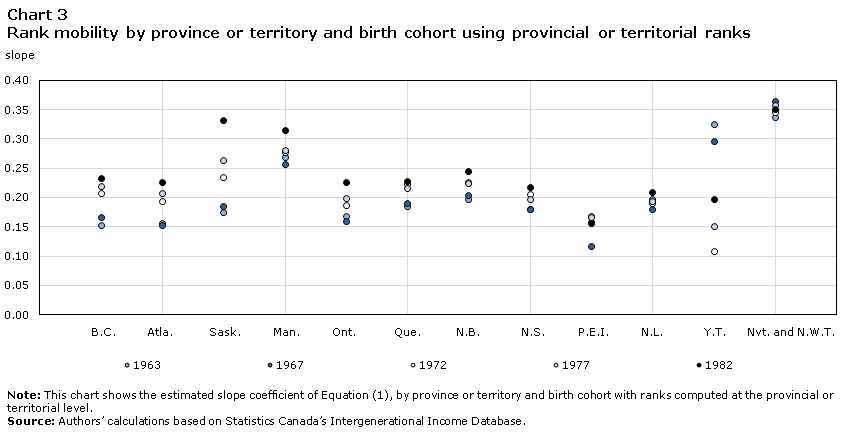
Thus far, the analysis has been at the national level. This subsection turns to intergenerational income mobility at the provincial and territorial level. Using provincial and territorial ranks is one way to consider the different circumstances in different provinces and territories and, in a sense, to control for cost of living differences. If a salary of $60,000 does not mean the same thing in Alberta and in Nova Scotia, then using within-province and within-territory ranks should help compare the relative positions of individuals in each. This is the approach used to generate the results shown in Chart 3.
Increases in the rank-rank slope are evidenced by the upward direction of the markers representing successive cohorts within each province and territory. Again, an increase in the rank-rank slope is indicative of declining intergenerational income mobility. In Ontario and Quebec, Canada’s two most populous provinces, the rank-rank slopes were respectively 0.058 and 0.043 points higher for the 1982 cohort compared to the 1963 cohort. In Saskatchewan, Alberta and British Columbia, the increases were 0.156, 0.070 and 0.080, respectively, representing percentage increases of 89%, 45% and 52%. Only Yukon shows an overall decrease in the rank-rank slope, but the population size is small compared with most other jurisdictions. Increases in rank-rank slopes were smaller in Atlantic Canada than other regions, suggesting that the prospects for intergenerational mobility are higher there. Yet, even so, the rank-rank slopes for the most recent cohorts were higher than those for previous cohorts, again suggesting declining mobility. The extent to which population mobility, particularly the outmigration of younger people from the region, affects these results is still to be determined. Provincial and territorial results using other measures, specifically after-tax income and parental and child rankings computed at the national level, are very similar to those in Chart 3.
Data table for Chart 3
| B.C. | Alta. | Sask. | Man. | Ont. | Que. | N.B. | N.S. | P.E.I. | N.L. | Y.T. | Nvt. and N.W.T. | |
|---|---|---|---|---|---|---|---|---|---|---|---|---|
| slope | ||||||||||||
| 1963 | 0.153 | 0.156 | 0.175 | 0.269 | 0.168 | 0.184 | 0.196 | 0.180 | 0.157 | 0.196 | 0.324 | 0.336 |
| 1967 | 0.166 | 0.152 | 0.184 | 0.256 | 0.159 | 0.190 | 0.203 | 0.180 | 0.116 | 0.179 | 0.295 | 0.364 |
| 1972 | 0.207 | 0.193 | 0.235 | 0.277 | 0.187 | 0.222 | 0.226 | 0.205 | 0.168 | 0.190 | 0.108 | 0.345 |
| 1977 | 0.218 | 0.207 | 0.263 | 0.281 | 0.199 | 0.215 | 0.224 | 0.196 | 0.166 | 0.193 | 0.150 | 0.357 |
| 1982 | 0.233 | 0.226 | 0.331 | 0.315 | 0.226 | 0.227 | 0.244 | 0.217 | 0.156 | 0.208 | 0.197 | 0.350 |
|
Note: This chart shows the estimated slope coefficient of Equation (1), by province or territory and birth cohort with ranks computed at the provincial or territorial level. Source: Authors' calculations based on Statistics Canada's Intergenerational Income Database. |
||||||||||||
3.4 Trends in transition matrices
In addition to rank-rank slopes and the IGE of income, transition matrices can be used to gauge intergenerational income mobility. In this subsection, data points from 5 x 5 transition matrices are presented, showing the probability of making a transition to a specific income quintile, conditional on the income quintile of one’s parents. Findings are presented graphically for ease of exposition. Chart 4 shows, conditional on the parental income quintile, the probability that a child has an income in the bottom quintile of their income distribution. For most parental income quintiles, this probability is relatively stable across the five birth cohorts, perhaps slightly decreasing in the top quintile. The largest movement is seen for children observed as teens in families at the bottom of the income distribution. the probability of remaining in the bottom quintile, increased from 0.27 to 0.33—a 22% increase—from the earliest to the most recent cohort. This suggests that it has become less likely for a child from the bottom income quintile to be in a higher quintile in their late 20s.

Data table for Chart 4
| Child's birth cohort | |||||
|---|---|---|---|---|---|
| 1963 | 1967 | 1972 | 1977 | 1982 | |
| probability of being in bottom quintile | |||||
| Quintile 1 (bottom) | 0.27 | 0.28 | 0.31 | 0.31 | 0.33 |
| Quintile 2 | 0.21 | 0.21 | 0.21 | 0.21 | 0.22 |
| Quintile 3 | 0.18 | 0.18 | 0.18 | 0.18 | 0.18 |
| Quintile 4 | 0.16 | 0.16 | 0.15 | 0.15 | 0.15 |
| Quintile 5 (top) | 0.15 | 0.15 | 0.14 | 0.14 | 0.13 |
|
Note: This chart shows the probability for a child to be in the bottom income quintile of their income distribution, by parental income quintile and birth cohort. Source: Authors’ calculations based on Statistics Canada’s Intergenerational Income Database. |
|||||
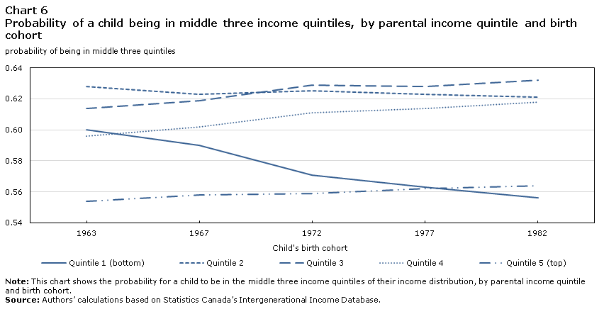
Chart 5 is constructed the same way as Chart 4 but shows the probability for a child to have an income in the top quintile of their distribution. Chart 5 shows that all the probabilities remain constant across the five birth cohorts. The flipside of the increase in observed in Chart 4 is therefore not that children from low-income families have had a lower probability of reaching the top income quintile over time, but rather that they have had a lower probability of being in one of the three middle income quintiles (quintiles 2, 3 or 4). This can be seen in Chart 6, which presents the probability for a child to be in those middle three quintiles, conditional on the parental income quintile. The drop in the transition into the middle three quintiles is clearly evident among children observed as teens in bottom-quintile families. For those children, the probability of reaching one of the three middle income quintiles declined from 0.60 for the 1963 birth cohort to 0.56 for the 1982 cohort, a decrease of just under 8%.

Data table for Chart 5
| Child's birth cohort | |||||
|---|---|---|---|---|---|
| 1963 | 1967 | 1972 | 1977 | 1982 | |
| probability of being in top quintile | |||||
| Quintile 1 (bottom) | 0.13 | 0.13 | 0.12 | 0.13 | 0.12 |
| Quintile 2 | 0.16 | 0.17 | 0.17 | 0.16 | 0.16 |
| Quintile 3 | 0.20 | 0.20 | 0.19 | 0.20 | 0.19 |
| Quintile 4 | 0.24 | 0.24 | 0.24 | 0.23 | 0.23 |
| Quintile 5 (top) | 0.30 | 0.29 | 0.30 | 0.30 | 0.30 |
|
Note: This chart shows the probability for a child to be in the top income quintile of their income distribution, by parental income quintile and birth cohort. Source: Authors’ calculations based on Statistics Canada’s Intergenerational Income Database. |
|||||
Data table for Chart 6
| Child's birth cohort | |||||
|---|---|---|---|---|---|
| 1963 | 1967 | 1972 | 1977 | 1982 | |
| probability of being in middle three quintiles | |||||
| Quintile 1 (bottom) | 0.60 | 0.59 | 0.57 | 0.56 | 0.56 |
| Quintile 2 | 0.63 | 0.62 | 0.63 | 0.62 | 0.62 |
| Quintile 3 | 0.61 | 0.62 | 0.63 | 0.63 | 0.63 |
| Quintile 4 | 0.60 | 0.60 | 0.61 | 0.61 | 0.62 |
| Quintile 5 (top) | 0.55 | 0.56 | 0.56 | 0.56 | 0.56 |
|
Note: This chart shows the probability for a child to be in the middle three income quintiles of their income distribution, by parental income quintile and birth cohort. Source: Authors’ calculations based on Statistics Canada’s Intergenerational Income Database. |
|||||
3.5 The Canadian Great Gatsby Curve
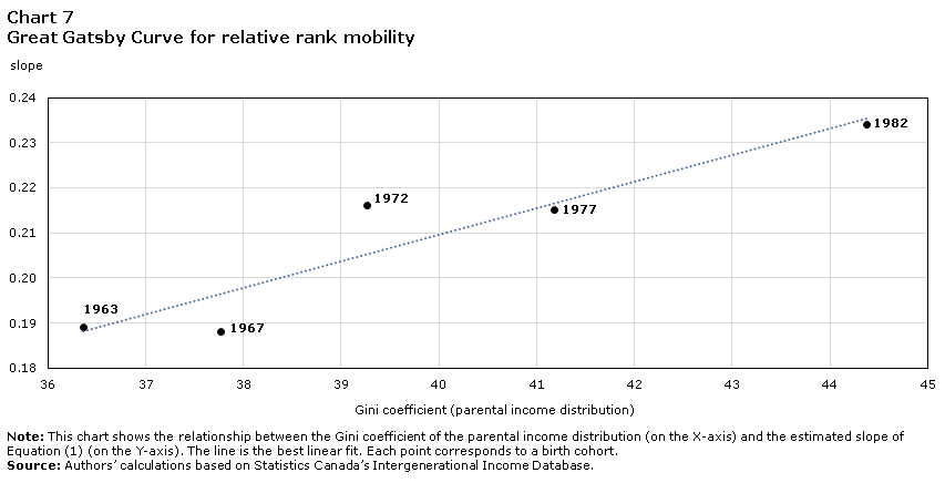
Now that measures of intergenerational income mobility have been presented for successive birth cohorts of Canadians, they can be charted along with parental income inequality, allowing Canada to be positioned on the Great Gatsby Curve. This is shown in Chart 7, which comprises the rank-rank slope—a measure of relative mobility—on the vertical axis and the Gini coefficient for parental income—a measure of inequality—on the horizontal axis. Each dot represents a birth cohort, as indicated. Over the span of these five cohorts, Canada has been “going up” the Great Gatsby Curve, characterized by an increasing degree of income inequality among parents and a decreasing degree of income mobility among children. This is consistent with the well-documented inequality–mobility relationship described in the international literature (Corak 2006, 2013) or within a country in a cross-sectional setting (Chetty et al. 2014a; Corak 2020). It indicates that the same relationship holds within a specific country across birth cohorts (i.e., over time). The results are much the same when the analysis is conducted using after-tax income. The Gini coefficients for the parental income distribution are lower when after-tax income is used—a result of the redistribution of income through the tax and transfer system—but the slope coefficients are very similar. The Great Gatsby Curve is thus simply shifted to the left (results not shown).
Data table for Chart 7
| Year | Slope | Gini coefficient |
|---|---|---|
| Gini coefficient | slope | |
| 1963 | 36.36 | 0.19 |
| 1967 | 37.77 | 0.19 |
| 1972 | 39.27 | 0.22 |
| 1977 | 41.18 | 0.22 |
| 1982 | 44.37 | 0.23 |
|
Note: This chart shows the relationship between the Gini coefficient of the parental income distribution (on the X-axis) and the estimated slope of Equation (1) (on the Y-axis). The line is the best linear fit. Each point corresponds to a birth cohort. Source: Authors’ calculations based on Statistics Canada’s Intergenerational Income Database. |
||
Charts 8a, 8b and 8c present the same information separately for each of the provinces this time. Each provincial series is labelled next to the point corresponding to the 1982 birth cohort, with earlier cohorts seen further down the line. The shift of most provinces up and to the right is indicative of movement up the Great Gatsby Curve, not just at the national level (as shown in Chart 7) but also at the provincial level. Some provinces have a relatively steep mobility–inequality profile, meaning that their decrease in mobility is relatively larger than their increase in inequality (e.g., Saskatchewan), while others have a flatter profile, with relatively large increases in inequality but not necessarily large increases in the rank-rank slope coefficient (e.g., Ontario).
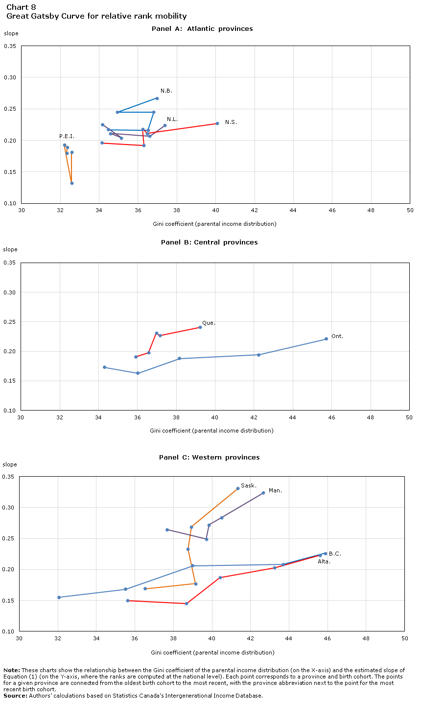
Data table for Chart 8
| Year | Gini | Slope | |
|---|---|---|---|
| Panel A: Atlantic provinces | |||
| N.B. | 1963 | 34.49 | 0.22 |
| 1967 | 36.51 | 0.22 | |
| 1972 | 36.80 | 0.25 | |
| 1977 | 34.94 | 0.25 | |
| 1982 | 36.97 | 0.27 | |
| N.L. | 1963 | 34.17 | 0.23 |
| 1967 | 35.14 | 0.20 | |
| 1972 | 34.57 | 0.21 | |
| 1977 | 36.60 | 0.21 | |
| 1982 | 37.38 | 0.22 | |
| N.S. | 1963 | 34.15 | 0.20 |
| 1967 | 36.30 | 0.19 | |
| 1972 | 36.24 | 0.22 | |
| 1977 | 36.48 | 0.21 | |
| 1982 | 40.07 | 0.23 | |
| P.E.I. | 1963 | 32.58 | 0.18 |
| 1967 | 32.58 | 0.13 | |
| 1972 | 32.20 | 0.19 | |
| 1977 | 32.35 | 0.19 | |
| 1982 | 32.32 | 0.18 | |
| Panel B: Central provinces | |||
| Ont. | 1963 | 34.32 | 0.17 |
| 1967 | 36.03 | 0.16 | |
| 1972 | 38.17 | 0.19 | |
| 1977 | 42.25 | 0.19 | |
| 1982 | 45.73 | 0.22 | |
| Que. | 1963 | 35.93 | 0.19 |
| 1967 | 36.57 | 0.20 | |
| 1972 | 36.97 | 0.23 | |
| 1977 | 37.14 | 0.23 | |
| 1982 | 39.23 | 0.24 | |
| Panel C: Western provinces | |||
| B.C. | 1963 | 32.07 | 0.16 |
| 1967 | 35.51 | 0.17 | |
| 1972 | 39.00 | 0.21 | |
| 1977 | 43.69 | 0.21 | |
| 1982 | 45.88 | 0.23 | |
| Alta. | 1963 | 35.63 | 0.15 |
| 1967 | 38.68 | 0.15 | |
| 1972 | 40.41 | 0.19 | |
| 1977 | 43.25 | 0.20 | |
| 1982 | 45.61 | 0.22 | |
| Sask. | 1963 | 36.53 | 0.17 |
| 1967 | 39.14 | 0.18 | |
| 1972 | 38.75 | 0.23 | |
| 1977 | 38.92 | 0.27 | |
| 1982 | 41.34 | 0.33 | |
| Man. | 1963 | 37.68 | 0.26 |
| 1967 | 39.70 | 0.25 | |
| 1972 | 39.84 | 0.27 | |
| 1977 | 40.50 | 0.28 | |
| 1982 | 42.66 | 0.32 | |
|
Note: These charts show the relationship between the Gini coefficient of the parental income distribution (on the X-axis) and the estimated slope of Equation (1) (on the Y-axis, where the ranks are computed at the national level). Each point corresponds to a province and birth cohort. The points for a given province are connected from the oldest birth cohort to the most recent, with the province abbreviation next to the point for the most recent birth cohort. Source: Authors’ calculations based on Statistics Canada’s Intergenerational Income Database. |
|||
3.6 Robustness analyses
Three robustness checks were undertaken for this analysis.
First, to address possible bias resulting from the fact that some individuals could be found in the tax files in only some years, the analysis was replicated on a restricted sample comprising only parents and children who were observed over the full five-year window during which income was measured. Results from this restricted sample largely replicate those from the main sample. For example, the estimated rank-rank slope went from 0.189 to 0.234 across birth cohorts in the main analysis and from 0.186 to 0.226 in the restricted set. Among children from the bottom parental income quintile, the rank-rank slope was actually higher in the restricted sample than the main sample, suggesting that the estimates above may be conservative. Overall, the potential bias from the unavailability of tax files for some individuals does not appear to diminish the results above.
A second robustness check was done using father’s income rather than total parental income in the analysis. Father’s income was tested to facilitate comparisons with the earlier literature, and because mother’s income can be less representative of the household’s place in the income distribution, given lower rates of female labour force participation. Although estimates of intergenerational income mobility are slightly lower when father’s income is used rather than parental income, the same upward trend remains. For example, the rank-rank slope increased from 0.158 to 0.183 over the period when father’s income was used, compared with an increase from 0.189 to 0.234 when parental income was used.
A third robustness check was done, in which the income measure for children was based on their family income in adulthood, defined as the sum of the income of the child and the income of their spouse, if present. Parental income is again defined as the total of both parents, if present. At ages 25 to 29, rank-rank slopes were only slightly lower using this approach than when individual child income was used. However, at older ages, the rank-rank slopes were higher when the child’s family income was used. This pattern is more pronounced for daughters than for sons, indicating that the inclusion of spouses’ income reinforces the intergenerational transmission of income, a finding that could be related to assortative mating. Further research in this direction warrants exploration.
4 Discussion and conclusion
In this study, decreases in social mobility across five consecutive birth cohorts in Canada are documented using a previously unavailable very large set of administrative tax files. The focus is on rank mobility, and findings show that the correlation between a child’s income rank as an adult and their parents’ income rank has been on an increasing trend, going from 0.189 to 0.234 between the 1963-to-1966 birth cohort and the 1982-to-1985 cohort. There also appears to be substantial nonlinearity in the rank mobility equation, motivating a split of the rank-rank slope in two segments: one for parental income rank up to the 20th percentile, the other for ranks 21 to 100. The bottom segment has much higher slopes, thus lower mobility, than the top segment. Moreover, the average child ranks for the more recent cohorts are lower than those of the first cohort for a substantial part of the bottom of the parental income distribution: even children whose parents are at the 30th to 35th percentiles have lower average ranks for the 1982-to-1985 cohort than for the 1963-to-1966 cohort.
Rank mobility is also described at the provincial and territorial levels. While there has been a deterioration of mobility in every single province, there are still large variations in rank-rank slopes across regions in the most recent cohort, and the within-province or within-territory variations over time have different magnitudes. Some places, notably the Atlantic provinces, have among the lowest rank-rank slopes, meaning the most equal opportunities for children, along with the smallest increases in slopes. Manitoba generally displays the lowest intergenerational mobility among the 10 provinces, and it is in Saskatchewan that the deterioration of equality of opportunities has been the worst. A look at quintile transition matrices reveals much the same story of declining mobility: children born in the bottom 20% of families in terms of income have become less likely to exit the bottom quintile themselves and less likely to transition into the middle class.
These results may seem to contradict Ostrovsky’s (2017) finding of stable rates of intergenerational income mobility between 1970 and 1984, using the same data source. However, Ostrovsky’s measure was quite different: he used as an absolute mobility measure the fraction of children earning more than their parents at age 30. This choice was motivated by the desire to compare the Canadian case with Chetty et al.’s (2017) similar estimates for the United States. Using income measured at age 30 for both parents and children constrained the cohorts that could be used from the IID. Because of data constraints, Ostrovsky’s analysis starts with birth year 1970, but the present analysis documents decreases in rank mobility starting with the 1963 birth cohort. It is possible that by having to start with the 1970 birth cohort, Ostrovsky’s analysis missed a substantial part of the decline observed herein. Moreover, the absolute mobility measure used in Ostrovsky’s analysis states which fraction of children tips past a certain income threshold. In so doing, it does not describe the rank-rank relationship at the same level of detail as done here.
Together with the increases in income inequality observed over the same time period, the increasingly strong association uncovered between parental income rank and child income rank means that Canada and every single province have been “going up” the Great Gatsby Curve. More inequality has gone hand in hand with lower mobility. This association is purely correlational at this stage, and the current descriptive analysis makes no attempt to uncover causal relationships. But the fact that the relationship holds across countries for a given time period, as well as for a given country over time and within a given country (across its regions) both at a given point in time and across time, points to something more than simply a spurious correlation.
Armed with a battery of descriptive statistics, a much clearer portrait of the situation of social mobility in Canada and its recent trends emerges. Many questions remain. What makes a region more mobile than another, and why do some experience much stronger declines? The empirical literature suggests some factors that correlate with more or less intergenerational income transmission (see Chetty et al. 2014a; Corak 2020; Connolly, Corak and Haeck 2019). Theoretical work also provides information on the various pathways that can shape human capital development and intergenerational transmission (see Heckman and Mosso 2014; Durlauf and Seshadri 2018; Bouchard St-Amant, Garon and Marceau 2020). But more research is needed to uncover causal mechanisms and identify public policies that may favour more equal opportunities for Canadian children, such as the work of Biasi (2019); Rothstein (2019); and Connolly, Haeck and Laliberté (2020).
References
Alvaredo, F., L. Chancel, T. Piketty, E. Saez, and G. Zucman, eds. 2018. World Inequality Report 2018. Belknap Press.
Biasi, B. 2019. School Finance Equalization Increases Intergenerational Mobility: Evidence from a Simulated-Instruments Approach. NBER Working Paper Series, no. w25600. Cambridge, Massachusetts: National Bureau of Economic Research.
Blanden, J. 2013. “Cross‐country rankings in intergenerational mobility: A comparison of approaches from economics and sociology.” Journal of Economic Surveys 27 (1): 38–73.
Bouchard St-Amant, P.-A., J.-D. Garon, and N. Marceau. 2020. Uncovering Gatsby Curves. CESifo Working Paper no. 8049 / Working Paper no. 2020-01. Montréal: Département des sciences économiques, École des sciences de la gestion, Université du Québec à Montréal.
Chen, W.H., Y. Ostrovsky, and P. Piraino. 2017. “Lifecycle variation, errors-in-variables bias and nonlinearities in intergenerational income transmission: New evidence from Canada.” Labour Economics 44 (January): 1–12.
Chetty, R., D. Grusky, M. Hell, N. Hendren, R. Manduca, and J. Narang. 2017. “The fading American dream: Trends in absolute income mobility since 1940.” Science 356 (6336): 398–406.
Chetty, R., N. Hendren, P. Kline, and E. Saez. 2014a. “Where is the land of opportunity? The geography of intergenerational mobility in the United States.” The Quarterly Journal of Economics 129 (4): 1553–1623.
Chetty, R., N. Hendren, P. Kline, E. Saez, and N. Turner. 2014b. “Is the United States still a land of opportunity? Recent trends in intergenerational mobility.” The American Economic Review 104 (5): 141–147.
Connolly, M., M. Corak, and C. Haeck. 2019. “Intergenerational mobility within and between Canada and the United States.” Journal of Labor Economics 37 (S2): S595–S641.
Connolly, M., C. Haeck, and J.-W. Laliberté. 2020. “Parental education and the rising transmission of income between generations.” In Measuring and Understanding the Distribution and Intra/Inter-Generational Mobility of Income and Wealth, ed. R. Chetty, J.N. Friedman, J.C. Gornick, B. Johnson, and A. Kennickell. NBER Book Series Studies in Income and Wealth. Chicago: University of Chicago Press. Forthcoming.
Corak, M. 2006. “Do poor children become poor adults? Lessons from a cross-country comparison of generational earnings mobility.” Research on Economic Inequality 13 (1): 143–188.
Corak, M. 2013. “Income inequality, equality of opportunity, and intergenerational mobility.” The Journal of Economic Perspectives 27 (3): 79–102.
Corak, M. 2020. “The Canadian geography of intergenerational income mobility.” The Economic Journal. Available at: https://doi.org/10.1093/ej/uez019.
Corak, M., and A. Heisz. 1999. “The intergenerational earnings and income mobility of Canadian men: Evidence from longitudinal income tax data.” Journal of Human Resources 34 (3): 504–533.
Dahl, M.W., and T. DeLeire. 2008. The Association Between Children’s Earnings and Fathers’ Lifetime Earnings: Estimates Using Administrative Data. Discussion Paper no. 1342-08. Institute for Research on Poverty, University of Wisconsin–Madison.
Davis, J., and B. Mazumder. 2017. The Decline in Intergenerational Mobility After 1980. Working Paper no. 2017-05. Chicago: Federal Reserve Bank of Chicago.
Durlauf, S.N., and A. Seshadri. 2018. “Understanding the Great Gatsby Curve.” In NBER Macroeconomics Annual 2017, ed. M.S. Eichenbaum and J. Parker, vol. 32. Chicago: University of Chicago Press.
Heckman, J.J., and S. Mosso. 2014. “The economics of human development and social mobility.” Annual Review of Economics 6 (1): 689–733.
Heisz, A. 2016. “Trends in income inequality in Canada and elsewhere.” In Income Inequality: The Canadian Story, ed. D.A. Green, W.C. Riddell, and F. St-Hilaire, p. 77–102. The Art of the State, vol. 5. Montréal: Institute for Research on Public Policy.
Ostrovsky, Y. 2017. Doing as Well as One’s Parents? Tracking Recent Changes in Absolute Income Mobility in Canada. Economic Insights, no. 73. Statistics Canada Catalogue no. 11-626-X. Ottawa: Statistics Canada.
Rothstein, J. 2019. “Inequality of educational opportunity? Schools as mediators of the intergenerational transmission of income.” Journal of Labor Economics 37 (S1): S85–S123.
Statistics Canada. 2016. “The rise of the dual-earner family with children.” Canadian Megatrends. Statistics Canada Catalogue no. 11-630-X. Ottawa: Statistics Canada.
- Date modified: