
Analytical Studies Branch Research Paper Series
Understanding Developments in Individuals’ Earnings Dispersion in Canada Using Matched Employer–Employee Data
Acknowledgements
The authors would like to thank Benoit Dostie from HEC Montréal, Danny Leung from Statistics Canada and Ben Tomlin from the Bank of Canada for their valuable comments and suggestions. The views expressed in this paper represent those of the authors only, not necessarily those of Statistics Canada or Finance Canada.
Abstract
This paper presents developments in the dispersion of individuals’ earnings in Canada and examines the potential of firm characteristics to account for this dispersion and changes in this dispersion. This paper uses the Canadian Employer–Employee Dynamics Database from 2001 to 2013 and shows that the overall earnings dispersion declined slightly over this time period, as the increasing dispersion in the top half of the distribution was offset by convergence in the bottom half. The increasing dispersion in the top half of the distribution is mostly attributable to the earnings of individuals in firms with 500 or more employees, while the decreasing dispersion in the bottom half occurred for workers in firms of all sizes. Evidence suggests that the rise in the minimum wage played a role in the decline in dispersion. Lastly, while both changes in earnings between industries and changes in the dispersion of productivity have an impact on the dispersion of individuals’ earnings, it has been found that the earnings dispersion within firms accounts for most of the dispersion in any given year and for all of the change across time.
Keywords: earnings, productivity, dispersion, inequality, matched employer–employee data.
Executive summary
The dispersion of earnings among workers may come from multiple sources. It may reflect differences in workers’ characteristics, such as education and experience. It may also be because workers are employed at different firms that pay differently. Recent studies from other countries have found that firms play an important role in explaining earnings disparities among workers, often through the link between productivity and pay. However, there has been no Canadian evidence on the link between the earnings dispersion and firm differences because of a lack of matched employer–employee data.
This paper presents developments in the dispersion of individuals’ earnings in Canada and examines the potential of firm characteristics to account for this dispersion and changes in this dispersion in the post-2000 period using the Canadian Employer–Employee Dynamics Database. The main findings can be summarized as follows.
First, consistent with other previous Canadian studies, this paper finds that the overall earnings dispersion in Canada has slightly declined over the 2001-to-2013 period. This was primarily because the earnings gain at the bottom of the earnings distribution outpaced the gain at the top. Specifically, while the upper half of the distribution (between the 90th and 50th percentiles) became more divergent throughout this period, the distribution in the bottom half (between the 50th and 10th percentiles) converged considerably faster. This decline in dispersion in the bottom half of the distribution was attributable to workers in firms of all sizes, while the increase in dispersion in the top half was mostly attributable to workers in large firms.
Second, the overall earnings dispersion declined within the provinces and territories, except for those most reliant on natural resources (i.e., Newfoundland and Labrador, Saskatchewan, Alberta, and British Columbia). Almost all provinces and territories experienced a decline in dispersion in the bottom half of the earnings distribution. All industrial sectors experienced decreases in the overall earnings dispersion and in the dispersion at the lower end of the distribution between 2001 and 2013. All sectors except utilities experienced an increase in the dispersion at the upper end.
Third, the evolving trends of the earnings distribution are quite different between male and female workers. Male workers experienced a large increase in the dispersion at the upper end of the distribution and a large decrease at the lower end, while female workers experienced a slight increase at the upper end and a slight decrease at the lower end. This is because male workers experienced a more pronounced polarization in earnings—both earnings at the top and the bottom of the distribution increased much faster than the median. For both men and women, evidence suggests that the increase in the minimum wage played a role in the decline of the dispersion in the bottom half of the distribution.
Fourth, decomposing the variance of earnings into within-firm and between-firm components shows that earnings differences within firms accounted for more than 60% of the overall dispersion in Canada, and that the decline in the within-firm dispersion accounted for the decline in the overall dispersion.
Firm characteristics have an impact on the earnings dispersion. Changes in the between-firm component of the earnings dispersion are the result of changes in between-firm earnings across industries, rather than within industries. The dispersion in firm productivity is positively related to the between-firm earnings dispersion at both the industry and firm levels. Moreover, larger or more productive firms experienced larger within-firm earnings dispersions.
1 Introduction
Inequality, no matter how it is measured, has generally increased since the late 1970s in Canada and in many other countries (see, for example, Katz and Murphy 1992; Katz and Autor 1999; Fortin et al. 2012; Heisz 2015; Card, Heining and Kline 2013; Song et al. 2019; Barth et al. 2016). Most previous studies have attributed this increase in inequality to (a) higher demand for skilled workers performing “abstract tasks” (requiring cognitive and interpersonal skills) induced by skill-biased technological change, which increases returns for more skilled workers (Autor, Levy and Murnane 2003; Autor, Katz and Kearney 2008; Autor and Acemoglu 2011); (b) a shortfall of investments in human capital and a failure to supply a sufficient number of high-skilled workers in response to skill-biased technological change (Murphy and Topel 2016); and (c) globalization and outsourcing that depress wages for middle- and low-skilled workers resulting from more competition with low-skilled, low-paid workers from developing countries (Autor, Dorn and Hanson 2013).
Recently, a new set of studies has attempted to assess the role of firms in explaining inequality.Note To that end, many studies have decomposed overall inequality into within-firm and between-firm components. Most of these studies used administrative data that link employers and workers and found that the increase in income disparity between firms has contributed significantly to the rise in overall inequality. For example, Song et al. (2019) looked at U.S. Social Security data and found that rising disparity in between-firm earnings accounted for more than two-thirds of the increase in the overall earnings inequality in the United States from 1981 to 2013. Similarly, Card, Heining and Kline (2013) looked at German social security data and found that increased differences in earnings among employers accounted for about one-third of the overall rise in inequality in Germany between 1985 and 2009. Lastly, Barth et al. (2016) looked at U.S. matched employer–employee data (the Longitudinal Employer-Household Dynamics database) and found that the widening distribution of earnings among establishments explained most of the increase in inequality.
The changing dispersion in average earnings between firms may reflect—in part—the change in worker composition between firms because of a sorting process that moves workers with similar skills into the same firms. It may also reflect the changing dispersion in productivity between firms that results from new technology, globalization or a change in market power, as productivity is often related to pay. Identifying trends in inequality and understanding the role firms play is important, as this can provide empirical evidence to inform public debate and guide policy. However, there has been no Canadian evidence on the link between earnings inequality and firm differences because of a lack of matched employer–employee data.Note Consequently, this paper provides empirical evidence on recent developments in Canadian earnings inequality after 2000, as well as their link to firm-level differences, particularly firm-level productivity. This analysis uses a newly developed matched employer–employee database: the Canadian Employer–Employee Dynamics Database (CEEDD). The CEEDD is particularly suitable for this study, as it covers all workers in Canada and their employers, and it also contains information on between-firm differences, including different measures of productivity.Note Therefore, this paper facilitates comparisons with other countries to determine whether Canada follows trends seen elsewhere or diverges from them.
Although inequality has been rising in Canada since the late 1970s, it has been stable and has even slightly declined since 2000 (Fortin and Lemieux 2015, and Heisz 2015).Note Consistent with these previous studies, this paper finds that the overall earnings dispersion (measured by the ratio of the 90th percentile of the earnings distribution to the 10th percentile) in Canada slightly declined between 2001 and 2013. This decline was mostly attributable to the earnings gain at the bottom of the earnings distribution outpacing that at the top, and this was closely related to the rise in minimum wages in Canada.
Decomposing the overall earnings dispersion into within-firm and between-firm components shows that the decline in the overall earnings dispersion was the result of a narrowing of the earnings differences within firms. The between-firm earnings dispersion increased slightly, driven solely by greater between-firm differences across industries, rather than within the same industry.
This study also finds that the dispersion in between-firm productivity increased between 2001 and 2013 and was positively related to the between-firm earnings dispersion at both the industry and firm levels. The findings on the relationship between differences in firm characteristics and the between-firm earnings dispersion are consistent with another Statistics Canada study (Grekou, Gu and Yan 2020), which also found that productivity and industrial differences played important roles.
The Canadian evidence presented in this study is generally consistent with that from other countries, such as the United States and other member countries of the Organisation for Economic Co-operation and Development (OECD): both dispersions in between-firm earnings and firm-level productivity increased in the post-2000 period and were positively correlated. However, the divergence of the between-firm earnings dispersion and the link between the productivity dispersion and the between-firm earnings dispersion were not as strong in Canada as they were in other countries.
This paper is organized as follows. Section 2 introduces the CEEDD and outlines the variables and methodology used to compute earnings, productivity and their dispersions. Section 3 presents the overall earnings dispersion in Canada, and the results on the within-firm and between-firm earnings dispersions are presented in Section 4. Section 5 examines the trend of firm-level productivity distribution over time, and its correlation to the earnings dispersion is examined in Section 6.
2 Data and methodology
The data source is the CEEDD, which is a Canadian matched employer–employee database. It is created by linking administrative data files, including individual tax files (T1 General – Income Tax and Benefit Return), individual employment remuneration files (T4 Statement of Remuneration Paid), incorporated (T2 Corporation Income Tax Return) and unincorporated business (T1 business declaration) tax files, and the Longitudinal Immigration Database (IMDB). The version of the CEEDD used in this study covers the annual universe of individual tax filers, as well as that of incorporated and unincorporated business tax filers in Canada from 2001 to 2013. The CEEDD is ideal for studying between-firm and within-firm earnings dispersions because it contains detailed information for all individual employees at a given firm, such as age, gender, marital status, immigrant status and job earnings. It is also ideal for studying the link between differences in earnings and productivity across firms because it contains information that can be used to calculate firm-level productivity, such as industry classification, number of employees, payroll, tangible assets, revenues, expenses and profits.
Several key concepts and variables are defined below in preparation for subsequent analysis. Earnings ( ) reflect workers’ total employment income from their main job in a given calendar year, as reported on their T4 slip.Note This means that, if a worker is employed by multiple firms in the same year, only the highest-paying firm (the main job) is used.Note It is important to note that this concept of earnings reflects total annual employment income rather than hourly wage. Therefore, patterns in the earnings dispersion could capture variations in both hourly wages and labour supply, such as the number of hours or weeks worked.Note The minimum earnings threshold is introduced later to reduce the impact of variation in hours worked.
Firm-level productivity is based on value added, which is measured as the sum of labour income and capital income. In the CEEDD, labour income is approximated by employment payroll and employee benefits, while capital income is approximated by total net income before tax.Note
Furthermore, two measures of firm-level productivity are used in this study: labour productivity ( ) and multifactor productivity ( ). LP, in a logarithm, is calculated as
where is firm ’s real value added in year , and is ’s employment as measured by ’s average monthly employment. MFP is calculated as the Solow residual, which, in a logarithm, is calculated as
where reflects ’s industry (classified using three-digit North American Industry Classification System [NAICS] code), is ’s real capital stock as per its book value of total tangible assetsNote and is industry ’s labour income share as measured by the median ratio of firm-level labour income to value added over the study period. Calculating MFP is straightforward, but it relies on the important assumption that production is characterized by a Cobb–Douglas function with constant returns to scale. Berlingieri, Blanchenay and Criscuolo (2017) found that the dispersion was fairly consistent across different measures of MFP, including the Solow residual. However, the correlation between the earnings dispersion and the MFP dispersion tends to be weaker when MFP is calculated using the Solow residual rather than with other measures.
Variance is used to measure dispersion in either earnings or firm-level productivity. Furthermore, the ratio between key percentiles in the distribution is used. The benefit of the latter measure is that it can show how different parts of a distribution behave. For example, while the ratio between the 90th and 10th percentiles (i.e., p90/p10) reflects overall dispersion, the ratios between the 90th and 50th (i.e., p90/p50) and the 50th and 10th (i.e., p50/p10) percentiles capture the dispersions in the upper and lower halves of the distribution, respectively.Note Following convention, earnings and productivity are often expressed as a logarithm. Therefore, the log of the ratio—or log differential (e.g., logp90-logp10)—is also used in the paper.
To construct the baseline sample for the analysis, several restrictions were applied. First, firm-level productivity was calculated only for incorporated firms in the business sector.Note In addition, productivity was measured only for firms that employed at least one worker on average throughout the year.
Second, restrictions were also applied to calculate the dispersion in earnings. The dispersion was based on the earnings of workers aged 20 to 60 to minimize the impacts of transitioning from school to work and from work to retirement.Note Moreover, workers in the baseline sample needed to earn at least the equivalent of 13 weeks of full-time work at the minimum wage of their province of residence.Note This restriction was imposed to reduce the effects of fluctuations in labour supply and the effects of workers who are weakly attached to the labour market. An alternative minimum earnings threshold (assuming full-time, full-year employment at minimum wage) was also used, and the impacts on the overall earnings dispersion remained qualitatively similar (see Chart A.1 in Appendix A). Lastly, a firm had to have at least five workers who satisfied the previous two conditionsNote to compute meaningful within-firm earnings variance.
In the end, the baseline sample accounts for one-third of all employers, but for a majority of total employment in the full sample that includes all workers who have positive earnings from any business (main jobs only) during a given year (Table B.1 in Appendix B). The full sample includes 661,500 to 916,900 firms that issued at least one T4 slip from 2001 to 2013 (Column 1). Each year, these firms employed about 12 million to 14 million individual workers (Column 2) and represented 9.7 million to 12 million in total employment as measured by PD7A average monthly employment (Column 3). The baseline sample consists of about 230,000 to 255,500 employers and about 8 million to 8.8 million individual workers each year (Columns 4 and 5), which respectively accounted for 32% of all employers and 62% of all workers in the full sample on average. However, the total employment associated with those employer firms in the baseline sample still ranged from about 8.4 million to 10 million, accounting for 85% of total employment in the full sample on average.
The earnings dispersions based on the baseline sample were qualitatively similar to those based on the full sample. This will be discussed in the next section.
3 Earnings dispersion in the post-2000 period
This section describes the earnings dispersion in Canada from 2001 to 2013 at the national level and by province, sector, firm size and gender.
3.1 National earnings dispersion
Chart 1 illustrates the trend in the various measures of the earnings dispersion in Canada from 2001 to 2013. More specifically, it shows how these measures have changed in year t from their respective values in 2001.
For the baseline sample, Chart 1 shows that the overall earnings dispersion—labelled “p90-p10”—increased until 2009 relative to its value in 2001. Specifically, overall inequality increased compared with its 2001 level and peaked in 2005. By this point, prior to the Great Recession, overall inequality was about 5% greater than in 2001.Note After 2005, the increase in overall inequality shrank until it was about 1% lower in 2013 than in 2001.
The overall decline in inequality occurred despite widening earnings gaps in the upper half of the distribution. Based on the baseline sample, the ratio between the 90th and 50th percentiles—labelled “p90-p50”—increased steadily and, by 2013, it was about 4% greater than in 2001. Overall inequality fell because declines in the dispersion in the lower half of the earnings distribution more than offset the increases in the top half. After rising moderately until 2004, the ratio between the 50th and 10th percentiles—labelled “p50-p10”—fell by about 5% by 2013.
It is important to emphasize that the sample restrictions imposed on the baseline sample do not seem to drive the observed trends in inequality. Chart 1 shows qualitatively similar results among a broader sample of workers (i.e., the full sample): overall inequality declined because the increase in the dispersion in the top half of the distribution was not large enough to offset the decrease in the dispersion in the lower half. However, one exception where restrictions do matter is with respect to the magnitudes of the decline in inequality: the full sample of workers yielded a larger decrease in inequality than the baseline sample. This is because the increase in dispersion in the top half of the earnings distribution was more modest in the full sample than in the baseline sample, while decreases in the lower half in both samples were of more similar magnitudes.

Data table for Chart 1
| Full sample | Baseline sample | |||||
|---|---|---|---|---|---|---|
| p90-p10 | p90-p50 | p50-p10 | p90-p10 | p90-p50 | p50-p10 | |
| change in dispersion (2001=0) | ||||||
| 2001 | 0.000 | 0.000 | 0.000 | 0.000 | 0.000 | 0.000 |
| 2002 | -0.002 | 0.006 | -0.008 | 0.020 | 0.006 | 0.014 |
| 2003 | 0.036 | 0.012 | 0.024 | 0.027 | 0.008 | 0.019 |
| 2004 | -0.001 | 0.009 | -0.009 | 0.042 | 0.019 | 0.022 |
| 2005 | 0.004 | 0.019 | -0.014 | 0.053 | 0.033 | 0.020 |
| 2006 | 0.002 | 0.021 | -0.020 | 0.047 | 0.037 | 0.011 |
| 2007 | 0.029 | 0.014 | 0.016 | 0.038 | 0.034 | 0.004 |
| 2008 | 0.013 | 0.002 | 0.010 | 0.025 | 0.032 | -0.007 |
| 2009 | -0.003 | -0.004 | 0.001 | 0.001 | 0.022 | -0.021 |
| 2010 | -0.041 | -0.001 | -0.040 | -0.002 | 0.031 | -0.033 |
| 2011 | -0.034 | 0.015 | -0.049 | -0.007 | 0.042 | -0.049 |
| 2012 | -0.024 | 0.014 | -0.038 | -0.014 | 0.042 | -0.056 |
| 2013 | -0.023 | 0.018 | -0.041 | -0.009 | 0.044 | -0.053 |
|
Notes: p90-p10 refers to the difference between the 90th and 10th percentiles of the log earnings distribution; p90-p50 refers to the difference between the 90th and 50th percentiles of the log earnings distribution; p50-p10 refers to the difference between the 50th and 10th percentiles of the log earnings distribution. Source: Statistics Canada, Canadian Employer–Employee Dynamics Database. |
||||||
As suggested by Fortin and Lemieux (2015), the decline in overall inequality and in the lower tail of the earnings distribution may be the result of increases in provincial minimum wages. Since 2005, minimum wage hikes could have made it possible for earnings at the bottom of the distribution to grow faster than those at the top or middle.Note Following Fortin and Lemieux (2015), the relationship between rising minimum wages and rising earnings at the bottom was examined. Estimation details are included in Appendix C. The results show that increases in the minimum wage led to increases in earnings at the bottom of the distribution. Moreover, the effect was more significant for female workers than male workers. This may be partly because there were proportionally more female workers who earned minimum wage or below (Fortin and Lemieux 2015), or because female workers who earned minimum wage wanted to work more hours, as increases in the minimum wage lead to an increase in the opportunity cost of leisure. Overall, this suggests that the rise in the minimum wage played a role in the decline of the dispersion at the bottom of the earnings distribution and, as a result, in the decline in the overall dispersion.
The slight decline—or relatively stable trend—in the overall earnings dispersion after 2000 is generally consistent with what has been found in other Canadian studies, such as those by Heisz (2015), who studied market income and after-tax income, and by Fortin and Lemieux (2015), who looked at hourly wages from the Labour Force Survey. This finding was also largely consistent with the overall earnings inequality trend in the United States after 2000, except that inequality in the United States increased again after the Great Recession (Song et al. 2019).Note
3.2 Other aspects of earnings dispersion
Are the trends observed at the national level widespread across geographic regions and sectors or are they specific to only a few provinces, territories or industries? Table 1 reports the change in the earnings dispersion from 2001 to 2013 for the baseline sample within each province or territory, sector, firm size category (measured by employment), and gender category.
Changes in the earnings dispersion between 2001 and 2013 were not uniform across provinces and territories (Panel A of Table 1). The overall earnings dispersion (p90/p10 ratio) declined within the territories and each province, except for those most reliant on natural resources (i.e., Newfoundland and Labrador, Saskatchewan, Alberta, and British Columbia). In most jurisdictions that experienced declines in the overall dispersion, these declines occurred at both the top and bottom of the distribution. Moreover, in these provinces, declines in the lower end of the distribution (p50/p10 ratio) were much larger than those in the upper end (p90/p50 ratio). For resource-rich provinces—except Newfoundland and Labrador—there were increases in overall inequality because of increases in the dispersion at the top of the distribution that offset decreases at the bottom. Most provinces and territories experienced a decline in the dispersion at the lower end of the distribution, although to varying degrees. As shown in the previous section, minimum wage was positively correlated with the 10th percentile of earnings, and this cross-province variation in the bottom half of the earnings dispersion may partially reflect the cross-province variation in the minimum wage and changes to the minimum wage over time.
Across economic sectors, changes in the earnings dispersion were more or less on par with the national trend, at least with respect to the direction of change (Panel B of Table 1). All sectors experienced decreases in the overall earnings dispersion (p90/p10 ratio) and in the dispersion at the lower end of the distribution (p50/p10 ratio) between 2001 and 2013. All sectors—except utilities—experienced an increase in the dispersion at the upper end, with the resources sector experiencing the highest increase in the p90/p50 ratio (7.5%), and manufacturing experiencing the lowest increase (1.2%), which is consistent with the economic development in these two sectors in the post-2000 period. At the same time, manufacturing had the largest decrease in the p50/p10 ratio (13.6%), which also led to the largest decrease in the overall earnings dispersion across sectors (12.5%).
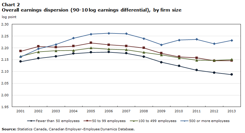
In terms of firm size, earnings inequality increased with firm size, especially between large firms (with 500 or more employees) and firms of all other sizes (Chart 2). This is consistent with Mueller, Ouimet and Simintzi (2017), who found that wage differentials between top- and bottom-level jobs and between different top-level jobs all increase with firm size.
Over time, workers in small and medium-sized firms (up to 499 employees) experienced a decrease in the overall earnings dispersion, while those in the largest firms (firms with at least 500 employees) experienced an increase of about 7.2% (Panel C of Table 1). All workers—except those in the smallest firms (fewer than 50 employees)—experienced an increase in the dispersion at the upper end of the distribution, which was also positively related to firm size. Workers in firms of all sizes experienced a decrease in the dispersion at the lower end of the earnings distribution.
Overall, the largest difference in the change in the earnings dispersion across firm-size categories was in the top half of the distribution, i.e., large firms (with 500 or more employees) experienced a large increase in the dispersion in the top half of the distribution, while smaller firms experienced a modest increase or decrease. This may be partly because large firms, which are usually more productive, have an increasing demand for more highly skilled workers, which inflates the skill premium.
| p90/p10 ratio | p90/p50 ratio | p50/p10 ratio | |
|---|---|---|---|
| percent | |||
| Panel A: Province or territory | |||
| Newfoundland and Labrador | 0.8 | -4.6 | 5.7 |
| Prince Edward Island | -5.7 | -1.4 | -4.3 |
| Nova Scotia | -15.2 | -5.0 | -10.7 |
| New Brunswick | -17.1 | -4.9 | -12.8 |
| Quebec | -2.7 | -0.4 | -2.3 |
| Ontario | -0.1 | 5.8 | -5.6 |
| Manitoba | -8.2 | 1.0 | -9.1 |
| Saskatchewan | 0.4 | 5.0 | -4.4 |
| Alberta | 2.1 | 5.9 | -3.6 |
| British Columbia | 4.3 | 6.7 | -2.2 |
| Northwest Territories, Yukon and Nunavut | -6.4 | -4.6 | -1.9 |
| Panel B: Sector | |||
| Agriculture | -10.0 | 1.8 | -11.6 |
| ResourcesTable 1 Note 1 | -2.9 | 7.5 | -9.7 |
| Utilities | -9.7 | -2.1 | -7.8 |
| Construction | -5.9 | 1.9 | -7.6 |
| Manufacturing | -12.5 | 1.2 | -13.6 |
| Services | -0.4 | 3.3 | -3.5 |
| Panel C: Firm size (employment) | |||
| Fewer than 50 employees | -5.4 | -1.5 | -3.9 |
| 50 to 99 employees | -4.0 | 1.5 | -5.4 |
| 100 to 499 employees | -1.3 | 3.5 | -4.7 |
| 500 or more employees | 7.2 | 10.1 | -2.6 |
| Panel D: Gender | |||
| All | -0.9 | 4.5 | -5.2 |
| Male | 1.2 | 7.3 | -5.7 |
| Female | 1.3 | 2.8 | -1.5 |
Source: Statistics Canada, Canadian Employer–Employee Dynamics Database. |
|||
Data table for Chart 2
| Firm size | ||||
|---|---|---|---|---|
| Fewer than 50 employees | 50 to 99 employees | 100 to 499 employees | 500 or more employees | |
| 2001 | 2.142 | 2.186 | 2.164 | 2.162 |
| 2002 | 2.156 | 2.206 | 2.183 | 2.196 |
| 2003 | 2.164 | 2.203 | 2.188 | 2.214 |
| 2004 | 2.176 | 2.207 | 2.189 | 2.241 |
| 2005 | 2.181 | 2.221 | 2.200 | 2.258 |
| 2006 | 2.182 | 2.213 | 2.195 | 2.262 |
| 2007 | 2.177 | 2.208 | 2.192 | 2.260 |
| 2008 | 2.163 | 2.200 | 2.181 | 2.239 |
| 2009 | 2.139 | 2.177 | 2.170 | 2.213 |
| 2010 | 2.123 | 2.162 | 2.158 | 2.233 |
| 2011 | 2.106 | 2.158 | 2.148 | 2.236 |
| 2012 | 2.095 | 2.145 | 2.147 | 2.217 |
| 2013 | 2.087 | 2.146 | 2.151 | 2.232 |
| Source: Statistics Canada, Canadian Employer–Employee Dynamics Database. | ||||
Both male and female workers experienced a similar and slight increase in the overall earnings dispersion (p90/p10 ratio) between 2001 and 2013 (Panel D of Table 1). However, the evolving trends of the earnings distribution are quite different between male and female workers. Male workers experienced a large increase in the dispersion at the upper end of the distribution and a large decrease at the lower end, while female workers experienced a slight increase at the upper end and a slight decrease at the lower end. This is because male workers experienced a pronounced polarization in earnings, as earnings at both the top and the bottom of the distribution increased much faster than the median (Chart 3). From 2001 to 2013, the earnings of male workers increased by 14% and 13% at the 90th and 10th percentiles, respectively, while earnings at the median grew by only 7%, which resulted in a convergence in the overall earnings dispersion. In contrast, female workers experienced similar growth at all three percentiles, 18%, 15% and 17% for the 90th, 50th and 10th percentiles, respectively. Compared with male workers, female workers experienced higher growth in all three percentiles, especially at the median (Chart 3).
When all workers (both male and female) were considered, the overall earnings distribution converged slightly. This is because of the composition effect, which results in the growth of both the top and the median earnings for all workers being disproportionally more affected by male workers, while the growth at the bottom of the distribution—especially at the 10th percentile—was more affected by female workers. This led to a more modest polarization in the earnings distribution for all workers than for male workers alone.Note

Data table for Chart 3
| Male workers | Female workers | |||||
|---|---|---|---|---|---|---|
| p90 | p50 | p10 | p90 | p50 | p10 | |
| 2001 | 1.000 | 1.000 | 1.000 | 1.000 | 1.000 | 1.000 |
| 2002 | 1.004 | 1.001 | 0.985 | 1.011 | 0.999 | 0.986 |
| 2003 | 1.000 | 0.991 | 0.972 | 1.010 | 1.001 | 0.976 |
| 2004 | 1.017 | 0.997 | 0.978 | 1.033 | 1.009 | 0.978 |
| 2005 | 1.038 | 1.001 | 0.987 | 1.038 | 1.012 | 0.979 |
| 2006 | 1.055 | 1.010 | 1.010 | 1.061 | 1.027 | 0.999 |
| 2007 | 1.073 | 1.019 | 1.031 | 1.086 | 1.057 | 1.024 |
| 2008 | 1.089 | 1.031 | 1.056 | 1.108 | 1.089 | 1.055 |
| 2009 | 1.080 | 1.020 | 1.046 | 1.127 | 1.118 | 1.096 |
| 2010 | 1.091 | 1.023 | 1.055 | 1.132 | 1.114 | 1.111 |
| 2011 | 1.104 | 1.027 | 1.079 | 1.140 | 1.112 | 1.128 |
| 2012 | 1.124 | 1.049 | 1.116 | 1.159 | 1.130 | 1.153 |
| 2013 | 1.144 | 1.066 | 1.130 | 1.184 | 1.152 | 1.169 |
|
Notes: p90 refers to the 90th percentile of the earnings distribution; p50 refers to the 50th percentile of the earnings distribution; p10 refers to the 10th percentile of the earnings distribution. Source: Statistics Canada, Canadian Employer–Employee Dynamics Database. |
||||||
4 Between-firm and within-firm earnings dispersions
The earnings dispersions shown in the previous section do not differentiate between workers within the same firm and those in different firms. This distinction is important because it can help better understand the role of firms in explaining the overall earnings inequality. According to the recent literature on this topic, within-firm earnings differences contribute to inequality differently than between-firm earnings differences. In particular, the literature documents that—in many countries—increases in between-firm earnings differences explain a large share of the rise in total inequality (e.g. Card, Heining and Kline 2013 for Germany; Faggio, Salvanes and Van Reenen 2010 and Mueller, Ouimet and Simintzi 2017 for United Kingdom; Barth et al., 2016 and Song et al., 2019 for the U.S.; and Helpman et al., 2017 for Brazil).Note However, there has been no Canadian evidence on this because of a lack of matched employer–employee data. This section decomposes the baseline sample’s total earnings variation into contributions from within-firm and between-firm variations.
To simplify the decomposition, earnings variance is used to measure inequality. This makes it easier for the earnings dispersion to be separated into between-firm and within-firm components as follows:
In Equation (1), is the earnings of worker at firm , is the average earnings in firm and is the average earnings for the entire sample, is the employment at firm , and is total employment of all firms in the sample. Given Equation (1), the overall variance in worker earnings equals the employment-weighted variance of firm-level average earnings (the first term on the right-hand side of Equation [1]) and the employment-weighted average variance of within-firm earnings (the second term on the right-hand side of Equation [1]).
Over the entire study period of 2001 to 2013, the contribution of the within-firm earnings variance to overall inequality was much greater than that of the between-firm variance. The within-firm variance accounted for more than 60% of the total earnings variance, on average. This variance also increased until 2007, but decreased thereafter. In contrast, the between-firm variance increased slightly. Between 2001 and 2013, the average within-firm variance decreased by 5.7%, while the between-firm variance increased by 2.8%. As a result, the total variance decreased by 2.5% from 2001 to 2013.

Data table for Chart 4
| Total variance | Between-firm variance | Within-firm variance | |
|---|---|---|---|
| variance | |||
| 2001 | 0.730 | 0.274 | 0.456 |
| 2002 | 0.738 | 0.279 | 0.459 |
| 2003 | 0.741 | 0.280 | 0.460 |
| 2004 | 0.752 | 0.285 | 0.467 |
| 2005 | 0.761 | 0.287 | 0.474 |
| 2006 | 0.760 | 0.284 | 0.476 |
| 2007 | 0.756 | 0.277 | 0.479 |
| 2008 | 0.742 | 0.272 | 0.470 |
| 2009 | 0.722 | 0.267 | 0.455 |
| 2010 | 0.721 | 0.272 | 0.449 |
| 2011 | 0.717 | 0.274 | 0.443 |
| 2012 | 0.709 | 0.276 | 0.434 |
| 2013 | 0.712 | 0.281 | 0.431 |
| Source: Statistics Canada, Canadian Employer–Employee Dynamics Database. | |||
This Canadian evidence on the evolution of within-firm and between-firm earnings variances after 2000 is qualitatively consistent with Song et al. (2019), who also found an increase in between-firm earnings variance and a decrease in within-firm earnings variance in the United States from 2000 to 2013. However, the increase in between-firm earnings variance was much larger in the United States, which led to an increase in the total earnings variance.Note
The between-firm earnings variance can be further decomposed into variance between firms in different groups (e.g., different industries) and variance between firms in the same group. The following equation shows this decomposition:
In Equation (2), is the specific earnings of worker in firm that belongs to group , is the average earnings of workers in , is the average earnings of workers in group , is firm ’s employment in group , is the number of firms in group , and is the total number of groups. Therefore, the total between-firm variance in Equation (1) can be fdecomposed into the variance of group-average earnings weighted by the group employment share (the first term on the right-hand side of Equation [2]) and the averageNote varianceNote in firm-level average earnings within each group (the second term on the right-hand side of Equation [2]).
The decomposition of the between-firm variations described by Equation (2) was implemented with respect to differences across industries (i.e., three-digit NAICS codes) and is illustrated in Chart 5. In terms of their levels, the between-industry and the within-industry, between-firm variations were of similar magnitude, each accounting for roughly 50% of the total between-firm variation in earnings.Note However, in terms of their changes, the between-industry variation was responsible for the overall increase in earnings variation between firms. Between 2001 and 2013, both the total between-firm and the between-industry firm variations in earnings first increased and then decreased to their lowest levels in 2009, before increasing again to end higher than in 2001. By contrast, the within-industry, between-firm variation increased until 2006, before declining until 2013 and ending at a slightly lower level than in 2001.

Data table for Chart 5
| Between-industry variance (left axis) | Within-industry, between-firm variance (left axis) | Total between-firm variance (right axis) | |
|---|---|---|---|
| variance | |||
| 2001 | 0.137 | 0.137 | 0.274 |
| 2002 | 0.139 | 0.140 | 0.279 |
| 2003 | 0.140 | 0.140 | 0.280 |
| 2004 | 0.143 | 0.142 | 0.285 |
| 2005 | 0.144 | 0.143 | 0.287 |
| 2006 | 0.140 | 0.143 | 0.283 |
| 2007 | 0.138 | 0.139 | 0.277 |
| 2008 | 0.135 | 0.138 | 0.273 |
| 2009 | 0.131 | 0.136 | 0.267 |
| 2010 | 0.136 | 0.137 | 0.273 |
| 2011 | 0.138 | 0.136 | 0.274 |
| 2012 | 0.141 | 0.135 | 0.276 |
| 2013 | 0.145 | 0.136 | 0.281 |
| Source: Statistics Canada, Canadian Employer–Employee Dynamics Database. | |||
In summary, the fall in overall inequality between 2001 and 2013 was primarily driven by the decline in the within-firm variance in earnings. The slight increase in between-firm earnings variance placed upward pressure on overall inequality and seems to have been driven entirely by a widening gap in the fortunes of workers in firms in different industries. Even though the earnings variance between firms within narrowly defined industries was considerable,Note this second source of inequality between firms declined between 2001 and 2013.
5 Firm-level productivity dispersion
As presented in previous sections, although the overall earnings dispersion declined, the between-firm variance in earnings widened slightly in Canada between 2001 and 2013. Diverging differences in firm performance could be the source of this inequality. Most prominently, firm productivity is generally positively correlated with average pay. If productivity differences between firms increase, more productive employers could pay their workers increasingly more than less productive firms. In fact, according to recent firm-level evidence, the dispersion of firm productivity increased in the post-2000 period in many OECD member countries where between-firm inequality also increased (Berlingieri, Blanchenay and Criscuolo 2017). This section explores the dispersion of firm-level productivity in Canada based on the sample of firms described in Section 2.
The overall dispersion of LP increased after 2001 in both the manufacturing and services sectors (Chart 6).Note The overall increase was accompanied in manufacturing by a slight decrease in the early 2000s and a slowdown after the 2008 financial crisis. A similar trend was also observed in the services sector. By 2013, the dispersion of LP—as measured by the ratio between the 90th and 10th percentiles—had increased by about 15%Note relative to its level in 2001. This increase was primarily driven by the increase in the dispersion at the upper rather than the lower part of the productivity distribution. LP was much more divergent in more productive firms (p90-p50) than in less productive firms (p50-p10) in both the manufacturing and services sectors. This differs from Berlingieri, Blanchenay and Criscuolo (2017), who found that the opposite was true in many other OECD member countries.
Dispersion trends for MFP (Chart 7) were similar to those for LP (Chart 6). The overall distribution of firm MFP increasingly diverged in the manufacturing and services sectors over time. Dispersion at both the top and bottom of the distribution also increased. Unlike LP (Chart 6), MFP became increasingly divergent in less productive firms (p50-p10) than in more productive firms (p90-p50) in the services sector.

Data table for Chart 6
| manufacturing sector | services sector | |||||
|---|---|---|---|---|---|---|
| p90-p10 | p90-p50 | p50-p10 | p90-p10 | p90-p50 | p50-p10 | |
| log point (2001=0) | ||||||
| 2001 | 0.000 | 0.000 | 0.000 | 0.000 | 0.000 | 0.000 |
| 2002 | 0.048 | 0.011 | 0.037 | 0.096 | 0.019 | 0.078 |
| 2003 | 0.050 | 0.013 | 0.037 | 0.133 | 0.035 | 0.098 |
| 2004 | 0.017 | 0.018 | -0.001 | 0.067 | 0.034 | 0.034 |
| 2005 | -0.009 | 0.001 | -0.011 | 0.084 | 0.058 | 0.026 |
| 2006 | 0.032 | 0.018 | 0.014 | 0.108 | 0.074 | 0.034 |
| 2007 | 0.054 | 0.038 | 0.017 | 0.112 | 0.075 | 0.038 |
| 2008 | 0.068 | 0.049 | 0.019 | 0.100 | 0.074 | 0.026 |
| 2009 | 0.110 | 0.063 | 0.047 | 0.078 | 0.060 | 0.019 |
| 2010 | 0.082 | 0.058 | 0.025 | 0.083 | 0.067 | 0.016 |
| 2011 | 0.077 | 0.065 | 0.012 | 0.095 | 0.083 | 0.012 |
| 2012 | 0.099 | 0.083 | 0.016 | 0.103 | 0.087 | 0.016 |
| 2013 | 0.142 | 0.102 | 0.039 | 0.138 | 0.104 | 0.034 |
|
Notes: p90-p10 refers to the difference between the 90th and 10th percentiles of the distribution of log labour productivity; p90-p50 refers to the difference between the 90th and 50th percentiles of the distribution of log labour productivity; p50-p10 refers to the difference between the 50th and 10th percentiles of the distribution of log labour productivity. Source: Statistics Canada, Canadian Employer–Employee Dynamics Database. |
||||||

Data table for Chart 7
| manufacturing sector | services sector | |||||
|---|---|---|---|---|---|---|
| p90-p10 | p90-p50 | p50-p10 | p90-p10 | p90-p50 | p50-p10 | |
| log point (2001=0) | ||||||
| 2001 | 0.000 | 0.000 | 0.000 | 0.000 | 0.000 | 0.000 |
| 2002 | 0.018 | 0.009 | 0.009 | 0.000 | -0.025 | 0.024 |
| 2003 | 0.040 | 0.013 | 0.027 | 0.040 | 0.000 | 0.040 |
| 2004 | 0.007 | 0.012 | -0.005 | 0.037 | 0.002 | 0.036 |
| 2005 | 0.039 | 0.033 | 0.006 | 0.105 | 0.063 | 0.043 |
| 2006 | 0.064 | 0.048 | 0.016 | 0.110 | 0.049 | 0.060 |
| 2007 | 0.106 | 0.064 | 0.042 | 0.128 | 0.065 | 0.062 |
| 2008 | 0.136 | 0.078 | 0.058 | 0.083 | 0.033 | 0.050 |
| 2009 | 0.172 | 0.082 | 0.090 | 0.076 | 0.041 | 0.035 |
| 2010 | 0.154 | 0.093 | 0.061 | 0.069 | 0.029 | 0.040 |
| 2011 | 0.146 | 0.102 | 0.044 | 0.100 | 0.007 | 0.093 |
| 2012 | 0.154 | 0.105 | 0.049 | 0.136 | 0.061 | 0.075 |
| 2013 | 0.178 | 0.119 | 0.059 | 0.140 | 0.057 | 0.083 |
|
Notes: p90-p10 refers to the difference between the 90th and 10th percentiles of the distribution of log multifactor productivity; p90-p50 refers to the difference between the 90th and 50th percentiles of the distribution of log multifactor productivity; p50-p10 refers to the difference between the 50th and 10th percentiles of the distribution of log multifactor productivity. Source: Statistics Canada, Canadian Employer–Employee Dynamics Database. |
||||||
6 The link between the earnings and productivity dispersions
As briefly described in the previous section, the firm productivity dispersion is expected to be positively correlated with the between-firm earnings dispersion. One possible explanation for this is that firms experiencing productivity increases because of technology adoption are likely to pass on some of these increases to their workers by increasing wages using rent-sharing mechanisms. This section formally examines the relationship between the earnings and productivity dispersions, with a focus on the correlation between the two, rather than on the causality.Note For this purpose, the following regression was estimated:
where measures the dispersion of firm-level earnings within industry (i.e., three-digit NAICS code) and in year , represents firm productivity dispersion, and and reflect year and industry fixed effects, respectively. Table 2 presents estimates of based on various measures of the earnings (columns) and productivity (rows) dispersions.
Column 1 shows that the overall dispersions in earnings and LP—each measured by the logged ratio of the 90th and 10th percentiles of their respective distributions—were positively correlated. Specifically, the estimated coefficient suggests that an increase of 1% in the dispersion of LP correlated with a 0.116% increase in the earnings dispersion.Note Table 2 also shows that the variance in earnings—as an alternative measure of the earnings dispersion—was positively and significantly correlated with the variance of LP (Column 4). The correlation coefficient was 0.107, which is only slightly smaller than the earnings dispersion measure used in Column 1.
The correlation between the earnings and productivity dispersions was also positive and significant at the top and bottom halves of the distributions (Columns 2 and 3), although it was stronger in the bottom half (Column 3). The weaker correlation in the top half of the distribution likely suggests that the firms at the top of the productivity distribution may pay top-level jobs excessively high wages relative to their productivity, in line with the recent theory on CEO compensation put forth by Gabaix and Landier (2008). Alternatively, the rise of “superstar firms” may reduce the bargaining power of workers in certain occupations, particularly for medium-skilled workers, whose pay may not fully reflect the productivity advantage of those firms (Autor et al. forthcoming).
The correlation between the earnings and MFP dispersions was also examined (Columns 5 to 8) and the results show that the link was not significant, except for in the bottom half of the distribution (Column 7). This may be because of the way the Solow-based MFP is constructed, which removes some heterogeneity across firms and relies on the assumption of constant returns to scale.Note
Overall, these results suggest that there is a positive co-movement between the LP and between-firm earnings dispersions. However, this link was weaker in Canada than in other OECD member countries (Berlingieri, Blanchenay and Criscuolo 2017). This could be partly attributable to differences in market competitiveness between Canada and other countries. According to the World Economic Forum (2020), Canada is ranked lower than most of the countries examined in the OECD study in terms of the product market index that measures the extent of market power, openness to foreign firms and degree of market distortions. A country with a less competitive market tends to have a weaker link between wages and productivity.
The correlation between the earnings and productivity dispersions can be further examined using firm-level data (i.e., regressing firm-level earnings against firm-level productivity), as illustrated in the following equation:
where is the firm-level average log earnings for firm in industry (i.e., three-digit NAICS code), region (census division), and time , is the corresponding firm-level productivity measure, measures the firm’s size in terms of employment, denotes the average log earnings across firms in the same industry and region as firm , and controls for firm-specific characteristics that do not change over time (i.e., firm fixed effects).
The key coefficient in Equation (4) is . This coefficient is often called the elasticity of rent sharing (see Card et al. [2018] for a review of the literature) and it measures the percentage change in firm-level earnings with respect to changes in firm productivity. The estimates of the elasticity of rent sharing are presented in Panel A of Table 3, where Column 1 shows the estimate of LP and Column 2 shows the estimate of MFP.
The rent-sharing—or pass-through—elasticity estimates presented in Table 3 show that firm-level earnings were positively correlated with firm-level productivity, even after controlling for firm size, average earnings in the same industry and region, and firm fixed effects (Columns 1 and 2). The estimates of LP and MFP suggest that, on average, a 1% increase in firm-level LP or MFP resulted in a 0.129% and 0.109% increase in firm-level average earnings, respectively. The magnitudes of these estimates are also comparable to estimates found in the literature (Card et al. 2018).Note
The estimated pass-through elasticity from productivity to earnings also suggests that, between 2001 and 2013, the rising dispersion of LP contributed to about 22% of the increase in the earnings dispersion between firms if all else remains the same.Note However, pass-through elasticity is assumed to be constant over time. Panel B of Table 3 reruns Equation (4) using an ordinary least squares regression separately for 2001 (Column 3) and 2013 (Column 4). The results show that pass-through elasticity decreased over time from 0.435 to 0.358, and the difference was significant at the 1% level. This suggests that, although firms became more divergent in terms of productivity, the productivity gains passed on to workers shrank over time. This placed downward pressure on the earnings inequality between firms.
This finding is consistent with another recent Canadian study that found that the pay premiums of frontier firms relative to non-frontier firms decreased over time (Grekou, Gu and Yan 2020).Note It is also consistent with a Brazilian study that found that declining firm productivity pay premiums contributed to the decrease in earnings inequality (Alvarez et al. 2018).
Equation (4) can be used to study how firm-level productivity affects the within-firm earnings dispersion. This is done by using the variance of logged earnings within the firm as the dependent variable. These results are presented in Panel C of Table 3.
Based on the estimates in Columns 5 and 6, it appears as if the within-firm earnings variation is also positively correlated with firm-level productivity, i.e., earnings tend to become more unequal within more productive firms. This may be in part because more productive firms are more likely to adopt performance-based pay policies that increase the variation of individual workers’ performance (Lazear 2000). Within-firm earnings variance is also positively related to firm size, after controlling for firm productivity. Earnings among workers tend to be more unequal within larger firms. This is consistent with Mueller, Ouimet and Simintzi (2017), who found that larger firms exhibited greater pay inequality in the United Kingdom. This was attributable not only to wage differences between the top-level and bottom-level jobs, but also to wage differences between different top-level jobs that increase with firm size.
| Productivity dispersion | Earnings dispersion | |||||||
|---|---|---|---|---|---|---|---|---|
| p90-p10 | p90-p50 | p50-p10 | Variance | p90-p10 | p90-p50 | p50-p10 | Variance | |
| Column 1 | Column 2 | Column 3 | Column 4 | Column 5 | Column 6 | Column 7 | Column 8 | |
| LP (p90-p10) | ||||||||
| Coefficient | 0.116Note ** | Note ...: not applicable | Note ...: not applicable | Note ...: not applicable | Note ...: not applicable | Note ...: not applicable | Note ...: not applicable | Note ...: not applicable |
| Standard error | 0.009 | Note ...: not applicable | Note ...: not applicable | Note ...: not applicable | Note ...: not applicable | Note ...: not applicable | Note ...: not applicable | Note ...: not applicable |
| LP (p90-p50) | ||||||||
| Coefficient | Note ...: not applicable | 0.088Note ** | Note ...: not applicable | Note ...: not applicable | Note ...: not applicable | Note ...: not applicable | Note ...: not applicable | Note ...: not applicable |
| Standard error | Note ...: not applicable | 0.011 | Note ...: not applicable | Note ...: not applicable | Note ...: not applicable | Note ...: not applicable | Note ...: not applicable | Note ...: not applicable |
| LP (p50-p10) | ||||||||
| Coefficient | Note ...: not applicable | Note ...: not applicable | 0.143Note ** | Note ...: not applicable | Note ...: not applicable | Note ...: not applicable | Note ...: not applicable | Note ...: not applicable |
| Standard error | Note ...: not applicable | Note ...: not applicable | 0.035 | Note ...: not applicable | Note ...: not applicable | Note ...: not applicable | Note ...: not applicable | Note ...: not applicable |
| Variance (LP) | ||||||||
| Coefficient | Note ...: not applicable | Note ...: not applicable | Note ...: not applicable | 0.107Note ** | Note ...: not applicable | Note ...: not applicable | Note ...: not applicable | Note ...: not applicable |
| Standard error | Note ...: not applicable | Note ...: not applicable | Note ...: not applicable | 0.014 | Note ...: not applicable | Note ...: not applicable | Note ...: not applicable | Note ...: not applicable |
| MFP (p90-p10) | ||||||||
| Coefficient | Note ...: not applicable | Note ...: not applicable | Note ...: not applicable | Note ...: not applicable | 0.035 | Note ...: not applicable | Note ...: not applicable | Note ...: not applicable |
| Standard error | Note ...: not applicable | Note ...: not applicable | Note ...: not applicable | Note ...: not applicable | 0.042 | Note ...: not applicable | Note ...: not applicable | Note ...: not applicable |
| MFP (p90-p50) | ||||||||
| Coefficient | Note ...: not applicable | Note ...: not applicable | Note ...: not applicable | Note ...: not applicable | Note ...: not applicable | -0.044 | Note ...: not applicable | Note ...: not applicable |
| Standard error | Note ...: not applicable | Note ...: not applicable | Note ...: not applicable | Note ...: not applicable | Note ...: not applicable | 0.029 | Note ...: not applicable | Note ...: not applicable |
| MFP (p50-p10) | ||||||||
| Coefficient | Note ...: not applicable | Note ...: not applicable | Note ...: not applicable | Note ...: not applicable | Note ...: not applicable | Note ...: not applicable | 0.166Table 2 Note † | Note ...: not applicable |
| Standard error | Note ...: not applicable | Note ...: not applicable | Note ...: not applicable | Note ...: not applicable | Note ...: not applicable | Note ...: not applicable | 0.100 | Note ...: not applicable |
| Variance (MFP) | ||||||||
| Coefficient | Note ...: not applicable | Note ...: not applicable | Note ...: not applicable | Note ...: not applicable | Note ...: not applicable | Note ...: not applicable | Note ...: not applicable | 0.041 |
| Standard error | Note ...: not applicable | Note ...: not applicable | Note ...: not applicable | Note ...: not applicable | Note ...: not applicable | Note ...: not applicable | Note ...: not applicable | 0.026 |
| Year fixed effect | Yes | Yes | Yes | Yes | Yes | Yes | Yes | Yes |
| Sector fixed effect | Yes | Yes | Yes | Yes | Yes | Yes | Yes | Yes |
| Number of observations | 1,209 | 1,209 | 1,209 | 1,209 | 1,209 | 1,209 | 1,209 | 1,209 |
| R-squared | 0.954 | 0.913 | 0.912 | 0.955 | 0.945 | 0.907 | 0.896 | 0.952 |
... not applicable
Source: Statistics Canada, Canadian Employer–Employee Dynamics Database. |
||||||||
| Variables | Panel A: Firm-level average earnings (fixed effect) | Panel B: Firm-level average earnings (OLS) | Panel C: Within-firm variance of logged earnings (fixed effect) |
|||
|---|---|---|---|---|---|---|
| 2001 to 2013 | 2001 to 2013 | 2001 | 2013 | 2001 to 2013 | 2001 to 2013 | |
| Column 1 | Column 2 | Column 3 | Column 4 | Column 5 | Column 6 | |
| ln(LP) | ||||||
| Coefficient | 0.129Note ** | Note ...: not applicable | 0.435Note ** | 0.358Note ** | 0.039Note ** | Note ...: not applicable |
| Standard error | 0.001 | Note ...: not applicable | 0.002 | 0.002 | 0.001 | Note ...: not applicable |
| ln(MFP) | ||||||
| Coefficient | Note ...: not applicable | 0.109Note ** | Note ...: not applicable | Note ...: not applicable | Note ...: not applicable | 0.034Note ** |
| Standard error | Note ...: not applicable | 0.001 | Note ...: not applicable | Note ...: not applicable | Note ...: not applicable | 0.001 |
| Size (log of employment) | ||||||
| Coefficient | 0.104Note ** | 0.081Note ** | 0.066Note ** | 0.068Note ** | 0.046Note ** | 0.040Note ** |
| Standard error | 0.001 | 0.001 | 0.001 | 0.001 | 0.000 | 0.001 |
| Average log earnings (industry–region level) | ||||||
| Coefficient | 0.105Note ** | 0.116Note ** | 0.251Note ** | 0.174Note ** | 0.020Note ** | 0.025Note ** |
| Standard error | 0.001 | 0.002 | 0.004 | 0.004 | 0.001 | 0.001 |
| Year fixed effect | Yes | Yes | No | No | Yes | Yes |
| Firm fixed effect | Yes | Yes | No | No | Yes | Yes |
| Industry fixed effect | No | No | Yes | Yes | No | No |
| Number of observations | 2,476,783 | 2,313,170 | 174,482 | 204,529 | 2,476,783 | 2,313,170 |
| R-squared | 0.885 | 0.883 | 0.621 | 0.622 | 0.574 | 0.572 |
... not applicable
Source: Statistics Canada, Canadian Employer–Employee Dynamics Database. |
||||||
7 Conclusion
Using new Canadian matched employer–employee data, this paper presents new evidence on the earnings dispersion from 2001 to 2013. It shows that the overall earnings dispersion declined slightly over the study period. This decline is attributable to the convergence of earnings in the bottom half of the distribution, which is closely related to the rise in the minimum wage in Canada during this period. It is also the result of the convergence of earnings in small and medium firms (with fewer than 500 employees), while the earnings dispersion among workers in large firms (500 employees or more) continued to rise.
This paper also differentiates between the between-firm and within-firm earnings dispersions. The results from this analysis indicate that the overall earnings dispersion declined because decreases in the within-firm dispersion more than offset slight increases in the between-firm dispersion. Moreover, the increasing between-firm earnings dispersion was found to be driven entirely by firms across industries rather than by firms within the same industry. This could mean that rising pay premiums in some Canadian industries (e.g., the resources and retail trade sectors) over the study period created positive pressure on inequality (Morissette, Picot and Lu 2013).
In terms of firm-level productivity, this study found that labour productivity (LP) and multifactor productivity became more divergent in Canada over time. This evidence is broadly consistent with that found in other countries. However, productivity in Canada became much more divergent among more productive firms than among less productive firms, unlike in other OECD member countries, where the opposite was found.
Lastly, this paper found a positive correlation between the LP and between-firm earnings dispersions and found that this correlation tended to be stronger in the bottom half of the distribution. The results from firm-level earnings regressions suggest that, although the increase in the between-firm earnings dispersion between 2001 and 2013 was small in magnitude, about 22% of this increase can be linked to a diverging firm-level LP dispersion. Moreover, the results also show that pass-through elasticity from productivity to earnings decreased over time. This suggests that, although firms became more divergent in terms of productivity, the productivity gains passed on to workers shrank over time, placing downward pressure on the earnings variation between firms.
The rising dispersion in average earnings between firms, coupled with the declining within-firm earnings dispersion, seems to support the theory that there is a sorting process through which workers with similar skills are moved into the same firms in the Canadian labour market. Future research using information from both workers and firms can shed more light on what underlies the earnings dispersion and its changes over time—whether that be differences between workers, differences between firms (including productivity and other traits), or the sorting of workers between firms that changes the composition of workers within and between firms.
Appendix A: Sensitivity analysis with different minimum earnings thresholds

Data table for Chart A.1
| 13 weeks worked | 52 weeks worked | |
|---|---|---|
| log point (2001=0) | ||
| 2001 | 0.000 | 0.000 |
| 2002 | 0.020 | 0.013 |
| 2003 | 0.027 | 0.019 |
| 2004 | 0.042 | 0.039 |
| 2005 | 0.053 | 0.057 |
| 2006 | 0.047 | 0.057 |
| 2007 | 0.038 | 0.061 |
| 2008 | 0.025 | 0.057 |
| 2009 | 0.001 | 0.017 |
| 2010 | -0.002 | 0.014 |
| 2011 | -0.007 | 0.002 |
| 2012 | -0.014 | 0.000 |
| 2013 | -0.009 | 0.002 |
| Source: Statistics Canada, Canadian Employer–Employee Dynamics Database. | ||
Appendix B: Sample coverage
| Full sample | Baseline sample | |||||
|---|---|---|---|---|---|---|
| Employers | Individual workers | Employment | Employers | Individual workers | Employment | |
| Column 1 | Column 2 | Column 3 | Column 4 | Column 5 | Column 6 | |
| number | ||||||
| 2001 | 661,500 | 12,455,300 | 9,651,600 | 229,600 | 7,988,400 | 8,357,200 |
| 2002 | 674,200 | 12,566,600 | 10,082,600 | 232,700 | 8,013,200 | 8,702,100 |
| 2003 | 692,600 | 12,740,700 | 10,335,100 | 238,300 | 8,189,300 | 8,945,400 |
| 2004 | 720,800 | 13,097,200 | 10,333,600 | 243,300 | 8,335,300 | 8,902,700 |
| 2005 | 735,100 | 13,304,300 | 10,545,700 | 245,400 | 8,461,000 | 9,077,200 |
| 2006 | 765,500 | 13,603,100 | 10,854,300 | 247,900 | 8,554,400 | 9,304,400 |
| 2007 | 799,300 | 14,255,800 | 11,443,100 | 252,500 | 8,736,000 | 9,602,300 |
| 2008 | 827,000 | 14,613,200 | 11,888,600 | 254,700 | 8,812,400 | 9,800,400 |
| 2009 | 838,400 | 14,324,600 | 11,553,100 | 252,700 | 8,503,000 | 9,456,700 |
| 2010 | 855,000 | 14,220,000 | 11,620,100 | 254,300 | 8,524,800 | 9,528,600 |
| 2011 | 874,400 | 14,136,000 | 11,521,200 | 254,800 | 8,598,600 | 9,692,900 |
| 2012 | 896,100 | 14,413,000 | 11,804,800 | 256,000 | 8,749,300 | 9,933,900 |
| 2013 | 916,900 | 14,617,700 | 12,010,100 | 255,500 | 8,796,200 | 10,035,900 |
| Source: Statistics Canada, Canadian Employer–Employee Dynamics Database. | ||||||
Appendix C: Estimating the relationship between minimum wages and earnings in the bottom half of the distribution
Following Fortin and Lemieux (2015), the following regression was estimated to assess the relationship between rising minimum wages and earnings in the bottom half of the distribution:
where denotes the earnings at a particular percentile , for province and year , is the earning at the median, is the provincial minimum earnings implied by the corresponding minimum wages at year , is a province-specific linear time trend, and and are province and year fixed effects, respectively. The left-hand side of the equation represents relative earnings, and on the right-hand side represents relative minimum earnings.
In theory, if the minimum wage is very low, it is not binding on the 10th percentile of wage distribution. As the minimum wage increases—and nears the 10th percentile—the slope on the 10th percentile ( in Equation (5) for a linear case) is expected to be positive because of spillover effects. If the minimum wage is equal to the 10th percentile, the slope should be equal to 1. As hourly wages are not available in the dataset, the minimum wages were replaced with the minimum earnings for each province, which are equal to province-specific minimum wages multiplied by 13 weeks and the national average of usual hours worked per week by full-time employees. However, the relationship between relative wage percentiles and relative minimum wage is expected to pass through to earnings.
Table C.1 shows the results for the relative earnings at the 10th percentile using both linear and quadratic specifications. The national average of usual hours worked per week was used to calculate the minimum earnings and year fixed effects were included in the regression, so the variation in is primarily the result of the variation in minimum wage. Therefore, the coefficients reflect the response of the earnings at the 10th percentile to the minimum wage. For all workers (male and female), the estimated coefficients are positive and significant under the linear specification (Column 1). Under the quadratic specification (Column 4), the response to the minimum wage is convex—as expected—and jointly significant. These results are consistent with those found by Fortin and Lemieux (2015) on the relationship between hourly wages and the minimum wage. This effect is more significant for female workers than for male workers (Column 2 versus Column 3, and Column 5 versus Column 6). This may be partly because there were proportionally more female workers who earned minimum wage or below (Fortin and Lemieux 2015), or because female workers who earned minimum wage wanted to work more hours as the minimum wage increased.
| Linear specification | Quadratic specification | |||||
|---|---|---|---|---|---|---|
| Both males and females | Males only | Females only | Both males and females | Males only | Females only | |
| Column 1 | Column 2 | Column 3 | Column 4 | Column 5 | Column 6 | |
| Relative minimum earnings | ||||||
| Coefficient | 0.467Note ** | 0.337Note ** | 0.527Note ** | 0.836 | 0.102 | 1.490Note ** |
| Standard error | 0.054 | 0.063 | 0.071 | 0.729 | 1.074 | 0.470 |
| Relative minimum earnings squared | ||||||
| Coefficient | Note ...: not applicable | Note ...: not applicable | Note ...: not applicable | 0.092 | -0.053 | 0.278Table C.1 Note † |
| Standard error | Note ...: not applicable | Note ...: not applicable | Note ...: not applicable | 0.179 | 0.245 | 0.140 |
| Province fixed effect | Yes | Yes | Yes | Yes | Yes | Yes |
| Year fixed effect | Yes | Yes | Yes | Yes | Yes | Yes |
| Joint test (p-value) | Note ...: not applicable | Note ...: not applicable | Note ...: not applicable | 0.000 | 0.002 | 0.000 |
... not applicable
|
||||||
References
Abowd, J., K. Mckinney, and N. Zhao. 2018. “Earnings inequality and mobility trends in the United States: Nationally representative estimates from longitudinally linked employer-employee data.” Journal of Labor Economics 36(s1): s183-s300.
Alvarez, J., F. Benguria, N. Engbom, and C. Moser. 2018. “Firms and the decline in earnings inequality in Brazil.” American Economic Journal: Macroeconomics 10 (1): 149–189.
Autor, D.H., and D. Acemoglu. 2011. “Skills, tasks and technologies: Implications for employment and earnings.” In Handbook of Labor Economics, ed. O. Ashenfelter and D. Card, volume 4B, p. 1043–1171. Amsterdam: Elsevier.
Autor, D.H., D. Dorn, and G.H. Hanson. 2013. “The China syndrome: Local labor market effects of import competition in the United States.” American Economic Review 103 (6): 2121–2168.
Autor, D.H., D. Dorn, L.F. Katz, C. Patterson, and J. Van Reenen. Forthcoming. “The fall of the labor share and the rise of superstar firms.” Quarterly Journal of Economics 135 (2).
Autor, D.H., L.F. Katz, and M.S. Kearney. 2008. “Trends in U.S. wage inequality: Revising the revisionists.” The Review of Economics and Statistics 90 (2): 300–323.
Autor, D.H., F. Levy, and R.J. Murnane. 2003. “The skill content of recent technological change: An empirical investigation.” The Quarterly Journal of Economics 118 (4): 1279–1333.
Barth, E., A. Bryson, J.C. Davis, and R. Freeman. 2016. “It’s where you work: Increases in earnings dispersion across establishments and individuals in the United States.” Journal of Labor Economics 34 (S2): S67–S97.
Berlingieri, G., P. Blanchenay, and C. Criscuolo. 2017. The Great Divergence(s). OECD Science, Technology and Innovation Policy Papers, no. 39. Paris: OECD Publishing.
Card, D., A.R. Cardoso, J. Heining, and P. Kline. 2018. “Firms and labor market inequality: Evidence and some theory.” Journal of Labor Economics 36 (S1): S13–S70.
Card, D., J. Heining, and P. Kline. 2013. “Workplace heterogeneity and the rise of West German wage inequality.” The Quarterly Journal of Economics 128 (3): 967–1015.
Employment and Social Development Canada. 2014. Historical minimum wage rates in Canada. Available at: https://open.canada.ca/data/dataset/390ee890-59bb-4f34-a37c-9732781ef8a0 (accessed January 23, 2020).
Faggio, G., K.G. Salvanes, and J. Van Reenen. 2010. “The evolution of inequality in productivity and wages: Panel data evidence.” Industrial and Corporate Change 19 (6): 1919–1951.
Fortin, N.M., D.A. Green, T. Lemieux, K. Milligan, and W.C. Riddell. 2012. “Canadian inequality: Recent developments and policy options.” Canadian Public Policy 38 (2): 121–145.
Fortin, N.M., and T. Lemieux. 2015. “Changes in wage inequality in Canada: An interprovincial perspective.” Canadian Journal of Economics 48 (2): 682–712.
Gabaix, X., and A. Landier. 2008. “Why has CEO pay increased so much?” The Quarterly Journal of Economics 123 (1): 49–100.
Grekou, D., W. Gu, and B. Yan. 2020. Decomposing the Between-firm Employment Earnings Dispersion in the Canadian Business Sector: The Role of Firm Characteristics.” Analytical Studies Branch Research Paper Series, no. 443. Statistics Canada Catalogue no.: 11F0019M. Ottawa: Statistics Canada.
Gu, W., B. Yan, and S. Ratté. 2018. Long-run Productivity Dispersion in Canadian Manufacturing. Economic Insights, no. 84. Statistics Canada Catalogue no. 11-626-X. Ottawa: Statistics Canada.
Heisz, A. 2015. “Trends in income inequality in Canada and elsewhere.” In Income Inequality: The Canadian Story, p. 77–102. Montréal: Institute for Research on Public Policy. Available at: http://irpp.org/research-studies/aots5-heisz/ (accessed January 23, 2020).
Helpman, E., O. Itskhoki, M.-A. Muendler, and S.J. Redding. 2017. “Trade and inequality: From theory to estimation.” The Review of Economic Studies 84 (1): 357–405.
Katz, L.F., and D.H. Autor. 1999. “Changes in the wage structure and earnings inequality.” In Handbook of Labor Economics, ed. O. Ashenfelter and D. Card, volume 3, p. 1463–1555. Amsterdam: Elsevier.
Katz, L.F., and K.M. Murphy. 1992. “Changes in relative wages, 1963–1987: Supply and demand factors.” The Quarterly Journal of Economics 107: 35–78.
Lazear, E.P. 2000. “Performance pay and productivity.” American Economic Review 90 (5): 1346–1361.
Morissette, R., G. Picot, and Y. Lu. 2013. The Evolution of Canadian Wages over the Last Three Decades. Analytical Studies Branch Research Paper Series, no. 347. Statistics Canada Catalogue no. 11F0019M. Ottawa: Statistics Canada.
Mueller, H.M., P.P. Ouimet, and E. Simintzi. 2017. “Wage inequality and firm growth.” American Economic Review: Papers & Proceedings 107 (5): 379–383.
Murphy, K.M., and R.H. Topel. 2016. “Human capital investment, inequality, and economic growth.” Journal of Labor Economics 34 (S2): S99–S127.
OECD (Organisation for Economic Co-operation and Development). 2019. “Workforce composition, productivity and pay: The role of firms in wage inequality developments.” Prepared for Working Party No. 1 of the Economic Policy Committee. Paris: Organisation for Economic Co-operation and Development.
Song, J., D. Price, F. Guvenen, N. Bloom, and T. Von Wachter. 2019. “Firming up inequality.” The Quarterly Journal of Economics 134 (1): 1–50.
Statistics Canada, Table 14-10-0043-01, Average usual and actual hours worked in a reference week by type of work (full- and part-time), annual. https://doi.org/10.25318/1410004301-eng.
Wooldridge, J.M. 2009. “On estimating firm-level production functions using proxy variables to control for unobservables.” Economics Letters 104 (3): 112–114.
World Economic Forum. 2020. The Global Competitiveness Report 2019. Available at: http://reports.weforum.org/global-competitiveness-report-2019/ (accessed January 23, 2020).
- Date modified: