
Analytical Studies Branch Research Paper Series
Decomposing the Between-firm Employment Earnings Dispersion in the Canadian Business Sector: The Role of Firm Characteristics
Abstract
This paper examines the role of firm characteristics in accounting for the between-firm average employment earnings dispersion in the Canadian business sector between 2002 and 2015. It uses two decomposition methods to analyze the level of and changes in the between-firm average employment earnings dispersion by firm characteristics, such as productivity, globalization status (importing, exporting, foreign ownership), technology intensity, firm size, firm age, industry and geographic region. The analysis shows that the between-firm average employment earnings dispersion has been declining at an annual rate of -0.09%, as measured by the mean logarithmic deviation dispersion index. The converging earnings between frontier and non-frontier firms account for about one-third of the aggregate decline. Converging earnings between industrial sectors and geographical regions are other important factors, contributing 9% and 7%, respectively, to the aggregate decline.
Keywords: earnings dispersion, productivity, globalization, technological change
JEL No.: D2, D3, F6, J3, O3
Executive summary
An extensive literature examines how the dispersion of individuals’ earnings has evolved over time. The literature examines whether these changes are attributed to changes in average earnings of workers with different characteristics (e.g., young versus old, male versus female and lower education versus higher education), or changes in workforce composition. The literature also recognizes that firm characteristics and the dispersion of average employment earnings between firms can play an important role in understanding the dispersion of individuals’ earnings.
This paper provides, for the first time, evidence for Canada on the dispersion of average employment earnings between firms, where the average employment earnings of a firm are calculated by dividing the firm’s annual payroll by the number of employees in a year. Specifically, this paper shows how the dispersion has changed over the 2002-2015 time period using several standard dispersion measures, and the contributions of firm characteristics in accounting for the dispersion at a point in time and to changes in the dispersion.
This study is relevant in the context of the increase in the relative productivity of the most productive firms compared with all other firms in Canada and in other member countries of the Organisation for Economic Co-operation and Development since 2000. Greater productivity dispersion among firms may lead to higher average employment earnings dispersion and more dispersion in individuals’ earnings.
This study finds that, when measured by the Gini coefficient, the dispersion in average employment earnings for firms is comparable in size to the income dispersion for individuals. Thus, changes in the between-firm earnings dispersion can be important in explaining the dispersion in individuals’ earnings.
This study finds that, when measured by the mean logarithmic deviation dispersion index, the percentage difference between the average employment earnings of a randomly selected firm and the average was 36.7% in 2015. The mean logarithmic deviation dispersion index is the focus of this study’s detailed analysis because it is a standard measure of dispersion, because the movements in the index are consistent with most of the other dispersion measures examined, and because it can be easily decomposed. Among the firm characteristics taken into account, differences in average employment earnings between frontier (the top 10th percentile of firms in terms of labour productivity) and non-frontier firms (all other firms), and between firms in different industries accounted for the largest shares (12.1% and 10%, respectively) of the 36.7%. The majority of the dispersion in average employment earnings was accounted for by dispersion within the different firm categories.
Several dispersion measures were also used to assess the change in dispersion over time, and the results vary depending on the measure used. Most of the measures tend to suggest that the dispersion in average employment earnings has not changed significantly, or has fallen slightly. Estimates range from a -0.7 to a 0.1 average annual percent change in dispersion over the period from 2002 to 2015. A decomposition of the -0.09 average annual percent change in the mean logarithmic deviation dispersion index between 2002 and 2015 shows that converging earnings between frontier and non-frontier firms explain roughly one-third of the decline—the largest fraction that can be associated with a firm characteristic when all characteristics are considered simultaneously.
Overall, the difference in average employment earnings between frontier and non-frontier firms is important in accounting for the dispersion and change in the dispersion in average employment earnings. These findings do not support the hypothesis that the growing productivity dispersion is leading to more earnings dispersion since average employment earnings between frontier and non-frontier firms are converging.
1 Introduction
In Canada, the earnings dispersion between workers rose from the 1970s to 2000, and has since remained stable.Note To study the patterns of earnings dispersion, researchers have focused on employee characteristics. For instance, the earnings dispersion in Canada was shown to be associated with earnings differences between older and younger workers (Morissette, Picot and Lu 2012), between workers with higher and lower education (Boudarbat, Lemieux and Riddell 2010), and between male and female workers (Baker and Drolet 2010). This paper takes a different approach and examines between-firm employment earnings dispersion and the role of firm characteristics in explaining the evolution of between-firm average employment earnings dispersion.
The literature provides evidence on the importance of between-firm effects in explaining total earnings dispersion. Barth et al. (2016) and Song et al. (2018) found that, in the United States, much of the increase in earnings dispersion among individuals since the 1970s was the result of increased earnings dispersion between firms, not increased earnings dispersion within firms. Dunne et al. (2004) reached a similar conclusion for manufacturing plants in the United States; using establishment-level data from 1975 to 1992, they argued that the between-plant component (within industries) of the total wage dispersion played the main role, and that its importance grew over the period examined. These results are consistent with those of Faggio, Salvanes and Van Reenen (2010), who found that, in the United Kingdom, the growth of between-firm dispersion (again, within industries) appeared to be the dominant reason for the increase in wage dispersion from 1984 to 2001. Alvarez et al. (2018) showed that firm effects accounted for 40% of the total decrease in earnings dispersion in Brazil between 1996 and 2012. The remainder came from worker effects (29%) and a weaker link between observable firm characteristics and worker pay (30%). Alvarez et al. (2018) also cited papers with similar conclusions about the importance of firm characteristics in explaining wage dispersion in Germany, Italy, Portugal, Brazil, Sweden and Denmark. Finally, Berlingieri, Blanchenay and Criscuolo (2017) emphasized that changes in between-firm dispersion played a significant part in the change in the overall earnings dispersion in member countries of the Organisation for Economic Co-operation and Development (OECD).
The drivers of between-firm effects have also received attention. Dunne et al. (2004) and Faggio, Salvanes and Van Reenen (2010) examined the role of skill-biased technical changes, whereby heterogeneous diffusion of new technology across firms and industries (e.g., uneven computer adoption) leads to a rise in the wages of skilled workers relative to unskilled workers. Fortin and Lemieux (2015) showed that the growth in the extractive resources sectors in Canada benefited less-educated and younger workers the most, and thereby reduced the wage dispersion in Newfoundland and Labrador, Saskatchewan, and Alberta. Goldschmidt and Schmieder (2015) looked at the outsourcing activity of firms (e.g., relying on contractors, temp agencies and franchises instead of hiring employees directly) and found that the outsourcing of cleaning, security and logistics services alone has accounted for around 10% of the increase in German wage dispersion since the 1980s.
This paper delves deeper into the contribution of firm characteristics to the dispersion of between-firm average employment earnings in Canada. It examines the underlying characteristics that have pulled firms apart or pushed them closer together in terms of average employment earnings. The evidence was established using linked firm microdata databases for the period from 2002 to 2015. Specifically, the core information on firms was obtained from Statistics Canada’s National Accounts Longitudinal Microdata File (NALMF) dataset. The NALMF allows to follow firms over time and contains key information—such as employment, earnings, industry and geography—and variables necessary to compute labour productivity. The NALMF was then linked to other firm microdata sources to obtain additional information, such as imports and exports (Canada Border Services Agency [CBSA] dataset for imports, Trade by Enterprise Characteristics [TEC] database, and Annual Survey of Manufactures [ASM] for exports) and foreign-ownership status (file from Statistics Canada’s Industrial Organization and Finance Division, supplemented by the Business Register File). Firms differ in productivity; participation in global production; intensity of technological change and investment; and other attributes such as size, age, industry and geographic location.
This analysis begins by showing trends in several standard dispersion indices, including the Gini coefficient, percentile ratios, generalized entropy (GE) indices (e.g., Theil’s L and T) and Atkinson indices. Despite differences between regions of the earnings distribution, these indices tend to suggest that the between-firm average employment earnings dispersion was stable and fell slightly at the national level between 2002 and 2015.
Next, the paper presents summary statistics on average employment earnings, the proportion of firms in the population, and within-group earnings dispersion by firm type. Firm types include frontier firms (defined as the top 10th percentile of firms in terms of labour productivity) versus non-frontier firms (all other firms), importers versus non-importers, exporters versus non-exporters, domestic-controlled versus foreign-controlled firms, capital intensity and research and development (R&D) intensity, firm age, firm size, industry, and location.
Two decomposition methods are then presented to quantify the contribution of firm characteristics to the evolution of between-firm average employment earnings dispersion. The first decomposition follows Jenkins (1995) and considers each firm’s characteristics separately. It examines how much of the total dispersion in between-firm average employment earnings is attributed to the dispersion within each group, and how much is attributed to earnings differences between groups. Next, a decomposition of the changes over time is implemented, following Mookherjee and Shorrocks (1982) and Jenkins (1995). Finally, to measure the contributions of all factors simultaneously, a second decomposition method that relies on a regression-based method (Fields 2003) is used.
The analysis shows that the between-firm average employment earnings dispersion has been declining at an annual rate of 0.09%, as measured by the mean logarithmic deviation dispersion index. All firm characteristics examined in this paper significantly affect the between-firm average employment earnings dispersion, but the converging earnings between the productivity frontier and non-frontier firms are the most important factor and explain approximately one-third of the aggregate decline.
The results suggest that the increasing productivity dispersion between frontier and non-frontier firms in Canada (Gu, Yan and Ratté 2018; Gu 2020) during the 2000s was not accompanied by a coinciding increase in the between-firm average employment earnings dispersion. This contrasts with evidence found for other OECD member countries (Berlingieri, Blanchenay and Criscuolo 2017). Two differences can be noted between the results for Canada and other OECD member countries. First, the between-firm average employment earnings dispersion has been stable and has declined slightly in Canada, but it has increased in the other countries.Note Second, the widening of the between-firm average employment earnings dispersion has been attributed to a widening of the productivity gap in other OECD member countries. This relationship is less clear in Canada, since these results suggest a convergence of average earnings between the productivity frontier and non-frontier firms.Note It should be noted, however, that evidence from other countries is mostly derived from an analysis of percentile ratios (i.e., a comparison of two specific points of the earnings distribution, such as the 90th and 10th percentiles, or the 50th and 10th percentiles), whereas this analysis takes the whole distribution into account.
This paper is organized as follows: Section 2 provides a description of the data sources and the classification of firm groupings. Section 3 presents the between-firm average employment earnings dispersion in Canada and statistics by firm groups. Section 4 outlines the two decomposition methods. Section 5 presents results of the decomposition methods. Section 6 concludes.
2 Data and summary statistics
2.1 Data sources and measurements
The data are mainly drawn from Statistics Canada’s NALMF for 2002 to 2015. The NALMF is an enterprise-level dataset that uses administrative tax records from the Canada Revenue Agency and data from the Business Register File. In each annual cross-section, the NALMF universe is defined as all enterprises in Canada that filed a Corporation Income Tax Return (T2), statements of remuneration paid (T4 slips), or Payroll Deduction Accounts (PD7). The file contains information on the core variables of interest for this study: total employment, earnings, labour productivity, capital intensity, R&D intensity, firm age, industry and province.
In this paper, the measure of total employment is the average monthly employment from the PD7, or the variable T4_ILU when the PD7 is missing.Note The labour cost is measured using payroll data from T4 slips, or payroll data from the PD7 when T4 slips are missing. Average employment earnings at the firm level are derived by dividing labour cost by total employment. Labour productivity is measured as value-added output divided by total employment, where value-added output is computed as the sum of profit (net income before tax) and labour cost.Note Labour productivity and employment earnings are all deflated by industry-level deflators derived from the Canadian Productivity Accounts.Note Capital intensity is calculated as total tangible assets (building, machinery and equipment) divided by total employment, and R&D intensity is calculated as total R&D expenditure divided by total employment. Finally, restrictions imposed on the dataset leave 11,860,773 observations in the analytical file from the NALMF.Note
Additional information on firm characteristics with respect to globalization indicators was also extracted for 2002 to 2015. Specifically, data on imports, exports and foreign ownership were retrieved from different sources. First, the total dollar value of imports was obtained from the CBSA dataset for each firm that could be matched in the NALMF. Second, the total dollar value of exports was extracted from two sources: the TEC database for 2010 to 2015, and the ASM for 2002 to 2009.Note Finally, information on whether firms were foreign-controlled or domestic-controlled was based on a special file from Statistics Canada’s Industrial Organization and Finance Division, supplemented by ownership information from the Business Register File. All datasets combined yield 11,802,300 observations, of which 1,414,358 have import values and 479,882 have export values.
2.2 Firm groups
The decomposition strategy adopted in this paper relies on distinguishing within-group and between-group effects. These firm groups are presented in Table 1 and include the following factors: productivity, three globalization indicators (importer, exporter, foreign ownership), two technology indicators (capital intensity and R&D intensity), firm size, firm age, industry and region. These groups cover an array of firm characteristics and have the advantage of being available in the analysis dataset.
| Potential factors | Decomposition groups | Definition |
|---|---|---|
| Productivity | Frontier versus non-frontier firms | 1 = Frontier firms (top 10th percentile of firms in terms of labour productivity in a year) 0 = Non-frontier firms (the remaining firms) |
| Globalization | Importers versus non-importers | 1 = Importer (firms with a positive value of imports) 0 = Non-importer (remaining firms) |
| Exporters versus non-exporters | 1 = Exporter (firms with a positive value of exports) 0 = Non-exporter (remaining firms) |
|
| Foreigned-controlled versus domestic | 1 = Foreign-controlled 0 = Domestic |
|
| Technology | Tangible capital per employee | 1 = Firms with intangible intensity greater than mean by year 0 = Firms with intangible intensity less than mean by year |
| Research and development per employee | 1 = Firms with research and development intensity greater than mean by year 0 = Firms with research and development intensity less than mean by year |
|
| Firm size | Firm size status | 1 = Small firms (0 to 99 employees) 2 = Medium firms (100 to 499 employees) 3 = Large firms (500 or more employees) |
| Age | Old versus young | 1 = Old (if age > mean age) by year 0 = Young (if age < mean age) by year |
| Industry | North American Industry Classification System two-digit level | 21 industries, excluding: Educational services (61) Health care and social assistance (62) Public administration (91) |
| Geographical | Provinces | 1 = Alberta 2 = British Columbia 3 = Manitoba 4 = New Brunswick 5 = Newfoundland and Labrador 6 = Nova Scotia 7 = Northwest Territories 8 = Nunavut 9 = Ontario 10 = Prince Edward Island 11 = Quebec 12 = Saskatchewan 13 = Yukon |
| Source: Statistics Canada. | ||
3 Trends in between-firm average employment earnings dispersion in Canada
This section serves as a base for the decomposition exercises that are implemented in the sections below. It summarizes the between-firm average employment earnings dispersion levels (overall and by firm grouping).
3.1 Between-firm average employment earnings dispersion
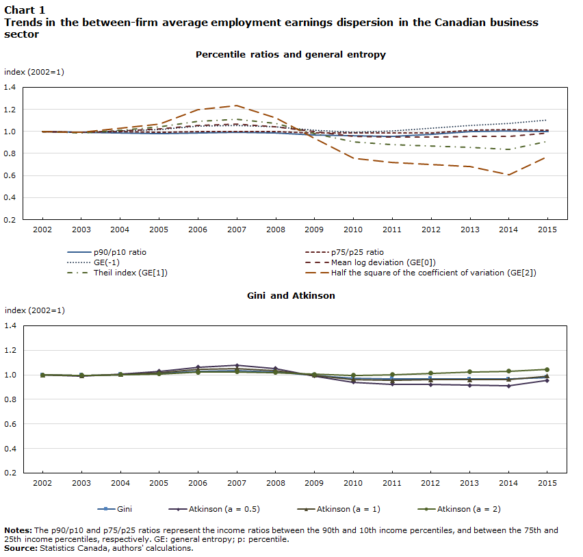
Economists regularly use a list of indices to measure income dispersion. These indices include the Gini coefficient, percentile ratios (e.g., p90/p10 and p75/p25), the GE class (GE[α] for α = -1, 0, 1, 2) and the Atkinson class (A[e], for e = 0.5, 1, 2). When the data described in Section 2 are used, 6 out of 10 dispersion indices concur in suggesting that between-firm average employment earnings dispersion was more or less stable from 2002 to 2015 (Chart 1 and Table 2). However, the preferred and most commonly used measure shows a slight decline in the employment earnings dispersion.
Data table for Chart 1
| p90/p10 ratio | p75/p25 ratio | GE(-1) | Mean log deviation (GE[0]) | Theil index (GE[1]) | Half the square of the coefficient of variation (GE[2]) | Gini | Atkinson (a = 0.5) | Atkinson (a = 1) | Atkinson (a = 2) | |
|---|---|---|---|---|---|---|---|---|---|---|
| index (2002=1) | ||||||||||
| 2002 | 1.00 | 1.00 | 1.00 | 1.00 | 1.00 | 1.00 | 1.00 | 1.00 | 1.00 | 1.00 |
| 2003 | 0.99 | 0.99 | 0.99 | 0.99 | 0.99 | 0.99 | 1.00 | 0.99 | 0.99 | 1.00 |
| 2004 | 0.98 | 1.00 | 1.01 | 1.00 | 1.01 | 1.03 | 1.00 | 1.01 | 1.00 | 1.00 |
| 2005 | 0.98 | 0.99 | 1.02 | 1.02 | 1.04 | 1.07 | 1.01 | 1.03 | 1.02 | 1.01 |
| 2006 | 0.99 | 1.00 | 1.05 | 1.05 | 1.09 | 1.19 | 1.03 | 1.06 | 1.04 | 1.02 |
| 2007 | 0.99 | 1.00 | 1.06 | 1.06 | 1.11 | 1.24 | 1.03 | 1.08 | 1.05 | 1.02 |
| 2008 | 0.99 | 1.00 | 1.04 | 1.04 | 1.07 | 1.12 | 1.02 | 1.05 | 1.04 | 1.02 |
| 2009 | 0.97 | 0.99 | 1.01 | 1.00 | 0.98 | 0.94 | 1.00 | 0.99 | 1.00 | 1.01 |
| 2010 | 0.96 | 0.98 | 0.99 | 0.96 | 0.90 | 0.76 | 0.98 | 0.94 | 0.96 | 1.00 |
| 2011 | 0.96 | 0.98 | 1.00 | 0.95 | 0.88 | 0.72 | 0.97 | 0.92 | 0.96 | 1.00 |
| 2012 | 0.97 | 0.99 | 1.03 | 0.95 | 0.87 | 0.70 | 0.97 | 0.92 | 0.96 | 1.01 |
| 2013 | 1.00 | 1.01 | 1.05 | 0.95 | 0.86 | 0.68 | 0.97 | 0.92 | 0.96 | 1.02 |
| 2014 | 1.01 | 1.01 | 1.07 | 0.95 | 0.84 | 0.61 | 0.97 | 0.91 | 0.96 | 1.03 |
| 2015 | 1.00 | 1.01 | 1.11 | 0.99 | 0.91 | 0.77 | 0.98 | 0.95 | 0.99 | 1.04 |
|
Notes: The p90/p10 and p75/p25 ratios represent the income ratios between the 90th and 10th income percentiles, and between the 75th and 25th income percentiles, respectively. GE: general entropy; p: percentile. Source: Statistics Canada, authors' calculations. |
||||||||||
| Indices | Level (indices × 100) | Average annual percent change, 2002 to 2005 |
|
|---|---|---|---|
| 2002 | 2015 | ||
| number | number | percent | |
| Income ratio: 90th versus 10th percentile | 700 | 701 | 0.01 |
| Income ratio: 75th versus 25th percentile | 271 | 274 | 0.09 |
| General entropy (-1) | 62 | 69 | 0.81 |
| Mean log deviation (general entropy [0]) | 37 | 37 | -0.09 |
| General entropy (1) | 46 | 42 | -0.69 |
| General entropy (2) | 187 | 144 | -1.75 |
| Gini | 45 | 44 | -0.15 |
| Atkinson (0.5) | 18 | 17 | -0.35 |
| Atkinson (1) | 31 | 31 | -0.08 |
| Atkinson (2) | 55 | 58 | 0.34 |
| Source: Statistics Canada, authors' calculations based on S.P. Jenkins, 1999, "INEQDECO: Stata module to calculate inequality indices with decomposition by subgroup." Statistical Software Components, no. S366002. | |||
On one hand, the percentile ratios (p90/p10 and p75/25) suggest a slight widening of the earnings gap between the top and bottom of the distribution (0.01% and 0.09% per year, respectively). This result aligns with findings for Canada from Gee, Liu and Rosell (2020), who used a percentile ratios definition and found an increase in between-firm dispersion from 2001 to 2013. This result is also consistent with the findings of Berlingieri, Blanchenay and Criscuolo (2017), which show a widening of the earnings dispersion for other OECD member countries. However, the limitation of the percentile ratios is that they report the earnings differences between specific segments of the distribution (e.g., earnings differences between the 90th and 10th percentiles). The percentile ratios are therefore easy to communicate, but do not reflect all changes in dispersion.
On the other hand, indices like the GE indices, the Atkinson indices and the Gini coefficient tend to indicate a slight narrowing of the between-firm average employment earnings gap. These indices have the advantage of responding to all changes in the earnings distribution, with varying sensitivity to different parts of the distribution (controlled by the parameters α for the GE and e for Atkinson).Note
For standard parameters, the analysis indicates a slight narrowing of the earnings gap (e.g., -0.09% for GE[0], -0.69% for GE[1], -0.15% for the Gini and -0.35% for A[0.5]). However, for extreme parameters that add sensitivity to the lower tail of the distribution (GE[-1]) or more aversion to dispersion (A[2]), the analysis suggests a widening of the earnings gap (0.81% per year for GE[-1] and 0.34% per year for A[2]). It should be noted that these trends are robust to the treatment of the outliers.Note
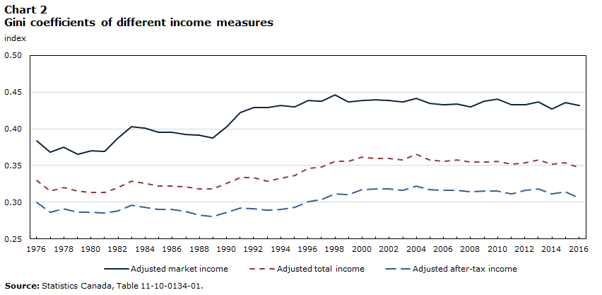
The suggested negative trend in this between-firm average employment earnings dispersion is consistent with evidence on aggregate earnings between workers. Indeed, between 1976 and 2016, the evolution of the Gini coefficients for market income, total income and after-tax income shares similar trends with that depicted here (Chart 2). A closer look at market income—the income concept that is closer to the definition used in this paper—shows two distinct periods: a period of rising dispersion from 1976 to 2000, followed by a period of relative decline in dispersion where the Gini coefficient fell but remained, within a narrow range, around the level reached in 2000. This result is also reported by Heisz (2016).
Data table for Chart 2
| Income concept | |||
|---|---|---|---|
| Adjusted market income | Adjusted total income | Adjusted after-tax income | |
| index | |||
| 1976 | 0.384 | 0.330 | 0.300 |
| 1977 | 0.368 | 0.315 | 0.286 |
| 1978 | 0.375 | 0.320 | 0.291 |
| 1979 | 0.365 | 0.315 | 0.286 |
| 1980 | 0.370 | 0.313 | 0.286 |
| 1981 | 0.369 | 0.313 | 0.285 |
| 1982 | 0.388 | 0.320 | 0.288 |
| 1983 | 0.403 | 0.329 | 0.296 |
| 1984 | 0.401 | 0.326 | 0.293 |
| 1985 | 0.395 | 0.322 | 0.290 |
| 1986 | 0.395 | 0.322 | 0.290 |
| 1987 | 0.392 | 0.321 | 0.287 |
| 1988 | 0.391 | 0.318 | 0.282 |
| 1989 | 0.388 | 0.318 | 0.281 |
| 1990 | 0.403 | 0.326 | 0.286 |
| 1991 | 0.422 | 0.334 | 0.292 |
| 1992 | 0.429 | 0.334 | 0.291 |
| 1993 | 0.429 | 0.329 | 0.289 |
| 1994 | 0.432 | 0.333 | 0.290 |
| 1995 | 0.430 | 0.336 | 0.293 |
| 1996 | 0.439 | 0.346 | 0.301 |
| 1997 | 0.438 | 0.348 | 0.304 |
| 1998 | 0.446 | 0.356 | 0.311 |
| 1999 | 0.437 | 0.356 | 0.310 |
| 2000 | 0.439 | 0.362 | 0.317 |
| 2001 | 0.440 | 0.360 | 0.318 |
| 2002 | 0.439 | 0.360 | 0.318 |
| 2003 | 0.437 | 0.358 | 0.316 |
| 2004 | 0.442 | 0.365 | 0.322 |
| 2005 | 0.435 | 0.358 | 0.317 |
| 2006 | 0.433 | 0.356 | 0.316 |
| 2007 | 0.434 | 0.358 | 0.316 |
| 2008 | 0.430 | 0.355 | 0.314 |
| 2009 | 0.438 | 0.355 | 0.315 |
| 2010 | 0.441 | 0.356 | 0.315 |
| 2011 | 0.433 | 0.352 | 0.311 |
| 2012 | 0.433 | 0.354 | 0.316 |
| 2013 | 0.437 | 0.358 | 0.318 |
| 2014 | 0.427 | 0.352 | 0.311 |
| 2015 | 0.436 | 0.354 | 0.314 |
| 2016 | 0.432 | 0.347 | 0.306 |
| Source: Statistics Canada, Table 11-10-0134-01. | |||
Following Jenkins (1995), the decomposition strategies in this paper use the GE(0)—also known as Theil’s L or the mean log deviation (MLD)—as described in Section 4 below. This is a standard measure of dispersion (Jenkins 1995; World Bank 2005) and, unlike the Gini coefficient, can be decomposed easily by firm group.
3.2 Summary statistics by firm group, industry and province
Table 3 shows the mean earnings relative to the Canadian average, the proportion of firms within each subgroup, and the earnings dispersion (as measured by the MLD). These are presented as an average over the period from 2002 to 2015 (left panel), and as an annual average rate of change between 2002 and 2015 (right panel).
The averages present three important facts. First, firms that have higher average employment earnings tend to be at the productivity frontier, globally connected (importers, exporters or foreign-controlled), technologically intensive (with higher capital or R&D intensity), older, larger or manufacturers. The differences in mean earnings are particularly large between frontier and non-frontier firms, and between foreign-controlled and domestic-controlled firms. The mean earnings for frontier firms are 3.9 times those of non-frontier firms, and the mean earnings for foreign-controlled firms are 2.1 times those of domestic-controlled firms.
Second, there are few high-wage firms: 12% for importers, 4% for exporters, 1% for foreign-controlled firms, 15% for firms with above-average capital intensity, 2% for firms with above-average R&D intensity, 1% for medium- to large-sized firms, and 6% for manufacturers.
Third, the between-firm average employment earnings dispersion within firms with high average employment earnings tends to be lower than that of their counterparts with low average employment earnings (0.8 times lower, on average). In other words, there seems to be less heterogeneity in average earnings at the top of the distribution. For example, the within-group earnings dispersion for exporters is about half that of non-importers. The two exceptions are frontier versus non-frontier firms (1.9 times more), and high-capital versus low-capital firms (1.1 times more).
Other important results from Table 3 pertain to the changes in average earnings between 2002 and 2015 (right panel). First, for a few categories, low-wage firms catch up to high-wage firms in mean earnings. The mean earnings of low-wage firms—such as non-frontier firms, non-importers, firms with low capital intensity, firms in non-manufacturing goods industries and firms in Atlantic Canada—have been growing faster than those of their respective counterparts. Second, while the overall between-firm average employment earnings dispersion decreased in Canada, it was not homogenous within groups. For example, it decreased for globally connected firms (-0.73% per year for importers, -1.98% per year for exporters, -0.78% per year for foreign-controlled firms), young firms (-0.76% per year), and small and medium-sized firms (-0.09% and -0.78% per year, respectively). However, the between-firm average employment earnings dispersion increased for frontier firms (+2.14% per year), old firms (+1.26% per year) and large firms (+0.80% per year). Therefore, the results show that both between-firm (e.g., catch-up) and within-firm factors have contributed to the general decline in the overall between-firm average employment earnings dispersion. However, these factors did not have homogenous effects across firm characteristics.Note
| Groups | Levels: averages from 2002 to 2015 | Annual average rate of change between 2002 and 2015 |
||||
|---|---|---|---|---|---|---|
| Mean earnings (relative to Canada average) | Proportion of firms |
Earnings dispersion within groupTable 3 Note 1 |
Mean earnings (relative to Canada average) | Proportion of firms |
Earnings dispersion within group |
|
| percent | number | percent change | percentage point |
percent change | ||
| Aggregate | 100.00 | 100.00 | 36.96 | 0.03 | 0.00 | -0.09 |
| Productivity | ||||||
| Non-frontier | 77.89 | 90.00 | 23.22 | 0.46 | 0.00 | 0.77 |
| Frontier | 300.20 | 10.00 | 44.85 | -0.88 | -0.01 | 2.14 |
| Globalization | ||||||
| Non-importers | 97.03 | 88.05 | 38.36 | 0.05 | -0.17 | 0.04 |
| Importers | 121.96 | 11.95 | 24.26 | -0.34 | 1.54 | -0.73 |
| Non-exporters | 97.46 | 96.19 | 36.59 | 0.19 | 0.06 | 0.19 |
| Exporters | 136.18 | 4.03 | 19.86 | 0.68 | -2.67 | -1.98 |
| Domestic-controlled | 99.36 | 99.42 | 36.81 | -0.01 | -0.04 | -0.13 |
| Foreign-controlled | 208.86 | 0.58 | 26.98 | 0.27 | 11.28 | -0.78 |
| Technology | ||||||
| Low capital intensity | 93.40 | 84.95 | 35.15 | 0.25 | 0.07 | 0.07 |
| High capital intensity | 137.15 | 15.05 | 40.23 | -0.63 | -0.41 | 0.03 |
| Low research and development intensity | 98.92 | 97.83 | 37.18 | 0.04 | 0.02 | -0.08 |
| High research and development intensity | 149.21 | 2.17 | 17.72 | 0.00 | -0.94 | -1.56 |
| Age | ||||||
| Young | 96.43 | 53.90 | 39.66 | -0.15 | -0.55 | -0.76 |
| Old | 104.00 | 46.10 | 33.40 | 0.21 | 0.79 | 1.26 |
| Firm size | ||||||
| Small | 99.68 | 98.73 | 37.08 | 0.02 | 0.00 | -0.09 |
| Medium | 121.67 | 1.07 | 24.80 | 0.74 | 0.09 | -0.78 |
| Large | 144.71 | 0.19 | 21.07 | 0.42 | 0.36 | 0.80 |
| Industry | ||||||
| Manufacturing | 104.36 | 5.81 | 21.13 | -0.13 | -1.97 | -0.82 |
| Non-manufacturing goods sector | 108.87 | 19.88 | 29.81 | 0.55 | 0.85 | -0.37 |
| Services | 97.26 | 74.32 | 39.93 | -0.13 | -0.03 | -0.09 |
| Region | ||||||
| Western Canada (B.C., Alta., Sask., Man.) |
110.36 | 36.32 | 42.33 | 0.44 | 0.59 | 0.62 |
| Central Canada (Ont., Que.) |
95.69 | 56.81 | 33.63 | -0.43 | -0.15 | -0.79 |
| Atlantic Canada (N.B., P.E.I., N.S., N.L.) |
79.27 | 6.57 | 29.42 | 1.32 | -1.57 | 0.49 |
| Northern Canada (Y.T., N.W.T., Nvt.) |
113.79 | 0.29 | 30.55 | 0.05 | -1.10 | -0.56 |
|
||||||
4 Analytical methods for decomposing earnings dispersion
The previous section showed the between-firm average employment earnings dispersion overall and by firm characteristics. This section explains the methodology used to quantify the contribution of firm characteristics to both the level of earnings dispersion across firms and the changes over time. Two decomposition methods are described. The first method decomposes the aggregate earnings dispersion in the Canadian business sector according to each of the characteristics discussed above (Table 1). The second decomposition method then uses regression-based techniques to measure the contributions of each factor simultaneously.
4.1 Decomposition by subgroup
One way to decompose the overall between-firm average employment earnings dispersion is to divide firms into various subgroups and to examine how much total dispersion is attributed to the inequalities within each subgroup and how much is attributed to the earnings differences between subgroups. Following Jenkins (1995), the MLD is used as the dispersion measure since it has the most desirable additive decomposability properties. The MLD formula is
where is the overall between-firm average employment earnings dispersion, µ is the average earnings among n firms, and Yi is the average employment earnings in firm i. The overall dispersion () can then be decomposed into within-group and between-group components:
where and , and and are the size and mean earnings of characteristic or subgroup g. The first term in Equation (2) is the within-group component, which is the weighted sum of dispersion within each subgroup, where the weights are the population share of each subgroup g. This is the part of that is due to dispersion within each subgroup or characteristic feature. The second term is the between-group component that measures dispersion arising from differences between subgroups if each subgroup member receives the mean earnings of their subgroup.
The decomposition strategy proposed by Mookherjee and Shorrocks (1982) and Jenkins (1995) is used to analyze the change in dispersion over time. The change in aggregate dispersion between t and t+1 is decomposed as follows:
where Δ is the difference between two years, and , and a bar above a variable indicates an average between the two years. Mookherjee and Shorrocks (1982) rewrote the last term in Equation (3) as
where , is group g’s share of total earnings, and the approximation is sufficient for computational purposes.Note The exact decomposition in Equation (3) can be computed with the approximation
[A] [B] [C] [D]
Equation (4) shows that changes in the overall between-firm average employment earnings dispersion between two years can be decomposed into four terms: pure dispersion changes within groups (A), changes attributed to shifts in firm demographics (different numbers of firms in different groups [B and C]) and changes attributed to shifts in the mean earnings of different groups (D). The changes in firm demographics reflect the changes in the population shares in the within-group component (term B) and the between-group component (term C).
To facilitate comparison across decompositions, the Jenkins (1995) method is used so that both sides of Equation (4) are divided by and the number of years to obtain proportionate average annual percent changes.
4.2 Regression-based decomposition
While the decomposition by subgroup provides a measure of dispersion between subgroups, it cannot tell which firm characteristics contributed the most to aggregate dispersion, especially when the factors are correlated. To determine which firm characteristics contributed the most to aggregate dispersion, the regression-based decomposition developed by Fields (2003) is used. It decomposes the overall between-firm average employment earnings dispersion to contributions accounted for by each factor. The method first estimates an income-generating function, such as
where Yit denotes the average employment earnings in firm i at time t, a set of k explanatory variables, βjt the coefficient associated with variable j at time t, and εit the error term. For each time t, it then estimates the share of the log-variance of earnings that is attributable to each factor (the relative factor dispersion weight), denoted by sjt as
where is the estimated coefficient from Equation (5), is the variance of the dependent variable, and is the covariance between the j th factor and the dependent variable at time t. The statistic sjt is comparable to the “between effect” found using the subgroup analysis. The sign of sjt indicates whether factor Xjt is dispersion-increasing (>0) or decreasing (<0).
It holds that
where R2 is the proportion of dispersion explained by the explanatory variable at time t, and sεt is the proportion unexplained by the explanatory variables included in the regression.
Fields (2003) extends the decomposition method to any dispersion index that is continuous, symmetric, and equal to zero when all incomes are equal. This therefore applies to the most common dispersion measures, including the MLD (Equation [1] above). Using the shares calculated in Equation (6), the change in dispersion attributed to factor Xj between time and can thus be derived as
To facilitate comparison across decompositions, Equation (8) is then divided by and the number of years to get contributions of each factor to the aggregate average annual percent changes.
5 Analytical results
5.1 Decomposition by subgroup
The first decomposition considers each firm characteristic separately and decomposes the overall between-firm average employment earnings dispersion into two components, as depicted in Equation (2) (Table 4). One component involves the inequalities within each subgroup (within-group component), and the second component involves the differences in average earnings between subgroups (between-group component). Given the exact decomposability property of the MLD, the sum of within-group and between-group components is equal to the total dispersion.
| 2002 | 2015 | |||||
|---|---|---|---|---|---|---|
| Total dispersion | Within-group component | Between-group component | Total dispersion | Within-group component | Between-group component | |
| number | ||||||
| Productivity | ||||||
| Frontier versus non-frontier firms | 37.17 | 24.05 | 13.11 | 36.71 | 27.14 | 9.57 |
| Globalization | ||||||
| Importers versus non-importers | 37.17 | 36.86 | 0.31 | 36.71 | 36.48 | 0.23 |
| Exporters versus non-exporters | 37.17 | 37.13 | 0.04 | 36.71 | 36.50 | 0.21 |
| Foreign-controlled versus domestic | 37.17 | 37.05 | 0.12 | 36.71 | 36.40 | 0.31 |
| Technology | ||||||
| High versus low capital intensity | 37.17 | 35.70 | 1.46 | 36.71 | 35.97 | 0.74 |
| High versus low research and development intensity | 37.17 | 36.96 | 0.20 | 36.71 | 36.54 | 0.17 |
| Age | ||||||
| Old versus young | 37.17 | 37.14 | 0.03 | 36.71 | 36.59 | 0.12 |
| Firm size | ||||||
| Small, medium and large | 37.17 | 37.14 | 0.03 | 36.71 | 36.66 | 0.05 |
| Region | ||||||
| 13 provinces and territories | 37.17 | 35.53 | 1.64 | 36.71 | 35.81 | 0.90 |
| Industry | ||||||
| 21 NAICS two-digit industries | 37.17 | 30.00 | 7.16 | 36.71 | 30.93 | 5.78 |
|
Notes: Dispersion is the mean logarithmic deviation. Estimates are based on Equation (2) in the text. Within- and between-group may not sum to aggregate dispersion because of rounding. Subgroups are defined in Table 1. For ease of presentation, the actual measured dispersion has been multiplied by 100. NAICS: North American Industry Classification System. Source: Statistics Canada, authors' calculations. |
||||||
The striking result from this decomposition of the between-firm average employment earnings dispersion is that, in both 2002 and 2015, the within-group component largely dominated the between-group component. Therefore, a large amount of between-firm average employment earnings variation remains unexplained by the firm characteristics examined. Productivity and industry differences are the only characteristics for which between-group differences explain an important part of the earnings dispersion. The differences in between-firm average earnings between frontier and non-frontier firms accounted for 35% and 26%, respectively, of the overall between-firm average earnings dispersion in 2002 and 2015. The between-group differences in the mean earnings across industries accounted for 19% and 16%, respectively, of the overall between-firm average employment earnings dispersion level in 2002 and 2015. For all other groups, the between-group component was low.
The second decomposition looks at the changes in the overall between-firm average employment earnings dispersion from 2002 to 2015 using Equation (4) (Table 5). The results show heterogeneity across groupings. For example, for four groupings (exporters versus non-exporters, foreign-controlled versus domestic-controlled, high R&D intensity versus low R&D intensity, and firm size), the within-group component (term A) was the most important term (accounting for 46%, 73%, 87% and 94%, respectively, of the changes in aggregate earnings for each grouping).Note For another four groupings (frontier versus non-frontier firms, high versus low capital, province and industry), the narrowing mean earnings between groups (term D) was the most important term (accounting for 53%, 64%, 39% and 43%, respectively, of the changes in the overall between-firm average employment earnings for each grouping). Finally, for the last two groupings (importers versus non-importers and old versus young), changes in demographics attributed to changes in the population shares on the within-group component (term B) was the most important term, accounting for about half of the changes in the overall between-firm average employment earnings dispersion.
| Change in aggregate dispersion | Changes in overall inequality accounted for by changes in | ||||
|---|---|---|---|---|---|
| Within-group dispersion | Population shares | Between-group dispersion | |||
| Within-group component | Between-group component | ||||
| ∆I | Term A | Term B | Term C | Term D | |
| percent change | |||||
| Frontier versus non-frontier firms | -0.09 | 0.64 | 0.00 | 0.00 | -0.73 |
| Importers versus non-importers | -0.09 | -0.02 | -0.06 | 0.01 | -0.03 |
| Exporters versus non-exporters | -0.09 | -0.08 | -0.05 | 0.01 | 0.03 |
| Foreign-controlled versus domestic | -0.09 | -0.13 | -0.01 | 0.04 | 0.00 |
| High versus low capital intensity | -0.09 | 0.06 | -0.01 | -0.01 | -0.14 |
| High versus low research and development intensity | -0.09 | -0.10 | 0.01 | 0.00 | 0.00 |
| Old versus young | -0.09 | -0.05 | -0.06 | 0.00 | 0.02 |
| Firm size (small, medium, large) | -0.09 | -0.10 | 0.00 | 0.00 | 0.01 |
| Region | -0.09 | -0.08 | 0.14 | -0.01 | -0.14 |
| Industry group (NAICS 2-digit industries) | -0.09 | 0.11 | 0.08 | -0.08 | -0.21 |
|
Notes: Subgroups are defined in Table 1. Terms ∆I, A, B, C and D are defined in Equation (4). Differences between ∆I and (A+B+C+D) are due to rounding. NAICS: North American Industry Classification System. Source: Statistics Canada, authors' calculations. |
|||||
These results show the relative importance of both within-group and between-group effects in explaining changes over time. They tend to suggest that shifts in firm demographics played a secondary role, except for the import and age groupings. This is different from other OECD member countries, where the between-group component seems to have been preponderant (Berlingieri, Blanchenay and Criscuolo 2017).
5.2 Regression-based decomposition
The regression-based decomposition relies on Equation (5) and considers all firm characteristics simultaneously to evaluate their relative contribution to the overall between-firm average employment earnings dispersion. The regressions are used to retrieve estimates (Tables 6-1 and 6-2) and to compute wage premiums (the anti-log of the estimates from Tables 6-1 and 6-2, and Table 7) for each year separately and for all years pooled together.
| Variables | 2002 | 2003 | 2004 | 2005 | 2006 | 2007 | 2008 | 2009 |
|---|---|---|---|---|---|---|---|---|
| Frontier firms | ||||||||
| Coefficient | 1.029Note ** | 1.018Note ** | 1.003Note ** | 0.993Note ** | 0.994Note ** | 0.981Note ** | 0.971Note ** | 0.951Note ** |
| Standard error | 0.003 | 0.003 | 0.003 | 0.003 | 0.003 | 0.003 | 0.003 | 0.003 |
| Importer | ||||||||
| Coefficient | 0.201Note ** | 0.188Note ** | 0.209Note ** | 0.238Note ** | 0.248Note ** | 0.247Note ** | 0.249Note ** | 0.248Note ** |
| Standard error | 0.003 | 0.003 | 0.003 | 0.003 | 0.003 | 0.003 | 0.003 | 0.003 |
| Exporter | ||||||||
| Coefficient | 0.088Note ** | 0.097Note ** | 0.148Note ** | 0.124Note ** | 0.126Note ** | 0.110Note ** | 0.089Note ** | 0.085Note ** |
| Standard error | 0.006 | 0.006 | 0.007 | 0.007 | 0.007 | 0.007 | 0.007 | 0.008 |
| Foreign-controlled | ||||||||
| Coefficient | 0.206Note ** | 0.191Note ** | 0.191Note ** | 0.196Note ** | 0.203Note ** | 0.225Note ** | 0.203Note ** | 0.211Note ** |
| Standard error | 0.014 | 0.014 | 0.013 | 0.012 | 0.012 | 0.010 | 0.010 | 0.010 |
| High capital intensity | ||||||||
| Coefficient | 0.210Note ** | 0.203Note ** | 0.193Note ** | 0.182Note ** | 0.177Note ** | 0.176Note ** | 0.174Note ** | 0.171Note ** |
| Standard error | 0.002 | 0.002 | 0.002 | 0.002 | 0.002 | 0.002 | 0.002 | 0.002 |
| High research and development intensity | ||||||||
| Coefficient | 0.246Note ** | 0.253Note ** | 0.242Note ** | 0.220Note ** | 0.236Note ** | 0.253Note ** | 0.255Note ** | 0.268Note ** |
| Standard error | 0.006 | 0.006 | 0.006 | 0.006 | 0.006 | 0.005 | 0.005 | 0.005 |
| Age—old firms | ||||||||
| Coefficient | 0.163Note ** | 0.154Note ** | 0.161Note ** | 0.147Note ** | 0.123Note ** | 0.115Note ** | 0.097Note ** | 0.104Note ** |
| Standard error | 0.002 | 0.002 | 0.002 | 0.002 | 0.002 | 0.002 | 0.002 | 0.002 |
| Firm size—medium | ||||||||
| Coefficient | 0.057Note ** | 0.068Note ** | 0.117Note ** | 0.089Note ** | 0.093Note ** | 0.087Note ** | 0.084Note ** | 0.086Note ** |
| Standard error | 0.008 | 0.007 | 0.008 | 0.008 | 0.008 | 0.008 | 0.008 | 0.008 |
| Firm size—large | ||||||||
| Coefficient | -0.009 | 0.007 | -0.020 | -0.040Table 6-1 Note † | -0.025 | -0.007 | -0.008 | -0.014 |
| Standard error | 0.018 | 0.018 | 0.018 | 0.018 | 0.018 | 0.018 | 0.018 | 0.018 |
| Fixed effects | ||||||||
| Region dummy variables | Yes | Yes | Yes | Yes | Yes | Yes | Yes | Yes |
| Industry dummy variables (NAICS 2-digit industries) | Yes | Yes | Yes | Yes | Yes | Yes | Yes | Yes |
| Year dummy variables | No | No | No | No | No | No | No | No |
| Number of observations | 771,915 | 772,714 | 804,958 | 818,080 | 839,014 | 859,341 | 858,017 | 850,385 |
| R-squared | 0.334 | 0.332 | 0.328 | 0.321 | 0.314 | 0.303 | 0.300 | 0.283 |
| Adjusted r-squared | 0.334 | 0.332 | 0.328 | 0.321 | 0.314 | 0.303 | 0.300 | 0.283 |
Source: Statistics Canada, authors' calculations. |
||||||||
| Variables | 2010 | 2011 | 2012 | 2013 | 2014 | 2015 | Pooled over all years (2002 to 2015) |
|---|---|---|---|---|---|---|---|
| Frontier firms | |||||||
| Coefficient | 0.907Note ** | 0.873Note ** | 0.858Note ** | 0.845Note ** | 0.825Note ** | 0.859Note ** | 0.934Note ** |
| Standard error | 0.003 | 0.003 | 0.003 | 0.003 | 0.003 | 0.003 | 0.001 |
| Importer | |||||||
| Coefficient | 0.236Note ** | 0.248Note ** | 0.250Note ** | 0.245Note ** | 0.248Note ** | 0.250Note ** | 0.240Note ** |
| Standard error | 0.003 | 0.003 | 0.003 | 0.003 | 0.003 | 0.003 | 0.001 |
| Exporter | |||||||
| Coefficient | 0.103Note ** | 0.113Note ** | 0.109Note ** | 0.103Note ** | 0.107Note ** | 0.115Note ** | 0.098Note ** |
| Standard error | 0.005 | 0.005 | 0.005 | 0.005 | 0.005 | 0.005 | 0.002 |
| Foreign-controlled | |||||||
| Coefficient | 0.199Note ** | 0.233Note ** | 0.254Note ** | 0.280Note ** | 0.310Note ** | 0.294Note ** | 0.227Note ** |
| Standard error | 0.010 | 0.010 | 0.010 | 0.010 | 0.010 | 0.010 | 0.003 |
| High capital intensity | |||||||
| Coefficient | 0.155Note ** | 0.155Note ** | 0.149Note ** | 0.157Note ** | 0.150Note ** | 0.149Note ** | 0.173Note ** |
| Standard error | 0.002 | 0.002 | 0.002 | 0.002 | 0.002 | 0.003 | 0.001 |
| High research and development intensity | |||||||
| Coefficient | 0.270Note ** | 0.279Note ** | 0.285Note ** | 0.295Note ** | 0.298Note ** | 0.285Note ** | 0.263Note ** |
| Standard error | 0.005 | 0.006 | 0.006 | 0.006 | 0.006 | 0.007 | 0.002 |
| Age—old firms | |||||||
| Coefficient | 0.100Note ** | 0.096Note ** | 0.093Note ** | 0.093Note ** | 0.093Note ** | 0.093Note ** | 0.113Note ** |
| Standard error | 0.002 | 0.002 | 0.002 | 0.002 | 0.002 | 0.002 | 0.000 |
| Firm size—medium | |||||||
| Coefficient | 0.093Note ** | 0.108Note ** | 0.112Note ** | 0.130Note ** | 0.150Note ** | 0.154Note ** | 0.107Note ** |
| Standard error | 0.008 | 0.008 | 0.008 | 0.008 | 0.008 | 0.008 | 0.002 |
| Firm size—large | |||||||
| Coefficient | -0.032Table 6-2 Note † | -0.038Note * | -0.011 | 0.020 | 0.036Table 6-2 Note † | 0.054Note ** | -0.003 |
| Standard error | 0.018 | 0.019 | 0.019 | 0.019 | 0.019 | 0.019 | 0.005 |
| Fixed effects | |||||||
| Region dummy variables | Yes | Yes | Yes | Yes | Yes | Yes | Yes |
| Industry dummy variables (NAICS 2-digit industries) | Yes | Yes | Yes | Yes | Yes | Yes | Yes |
| Year dummy variables | No | No | No | No | No | No | Yes |
| Number of observations | 859,574 | 865,263 | 872,951 | 875,835 | 886,602 | 867,651 | 11,802,300 |
| R-squared | 0.264 | 0.248 | 0.234 | 0.236 | 0.227 | 0.230 | 0.276 |
| Adjusted r-squared | 0.264 | 0.248 | 0.234 | 0.236 | 0.227 | 0.230 | 0.276 |
Source: Statistics Canada, authors' calculations. |
|||||||
| Variables | 2002 | 2003 | 2004 | 2005 | 2006 | 2007 | 2008 | 2009 | 2010 | 2011 | 2012 | 2013 | 2014 | 2015 | Pooled over all years | Average annual percent change |
|---|---|---|---|---|---|---|---|---|---|---|---|---|---|---|---|---|
| number | percent | |||||||||||||||
| Frontier firms relative to non-frontier firms | 2.80 | 2.77 | 2.73 | 2.70 | 2.70 | 2.67 | 2.64 | 2.59 | 2.48 | 2.39 | 2.36 | 2.33 | 2.28 | 2.36 | 2.54 | -0.70 |
| Importers relative to non-importers | 1.22 | 1.21 | 1.23 | 1.27 | 1.28 | 1.28 | 1.28 | 1.28 | 1.27 | 1.28 | 1.28 | 1.28 | 1.28 | 1.28 | 1.27 | 0.31 |
| Exporters relative to non-exporters | 1.09 | 1.10 | 1.16 | 1.13 | 1.13 | 1.12 | 1.09 | 1.09 | 1.11 | 1.12 | 1.11 | 1.11 | 1.11 | 1.12 | 1.10 | 0.08 |
| Foreign-controlled firms relative to domestic firms | 1.23 | 1.21 | 1.21 | 1.22 | 1.22 | 1.25 | 1.23 | 1.23 | 1.22 | 1.26 | 1.29 | 1.32 | 1.36 | 1.34 | 1.25 | 0.16 |
| High capital intensity firms relative to low capital intensity firms | 1.23 | 1.23 | 1.21 | 1.20 | 1.19 | 1.19 | 1.19 | 1.19 | 1.17 | 1.17 | 1.16 | 1.17 | 1.16 | 1.16 | 1.19 | -0.28 |
| High research and development intensity firms relative to low research and development intensity firms | 1.28 | 1.29 | 1.27 | 1.25 | 1.27 | 1.29 | 1.29 | 1.31 | 1.31 | 1.32 | 1.33 | 1.34 | 1.35 | 1.33 | 1.30 | 0.13 |
| Old firms relative to young firms | 1.18 | 1.17 | 1.17 | 1.16 | 1.13 | 1.12 | 1.10 | 1.11 | 1.11 | 1.10 | 1.10 | 1.10 | 1.10 | 1.10 | 1.12 | -0.38 |
| Medium-sized firms relative to small firms | 1.06 | 1.07 | 1.12 | 1.09 | 1.10 | 1.09 | 1.09 | 1.09 | 1.10 | 1.11 | 1.12 | 1.14 | 1.16 | 1.17 | 1.11 | 0.39 |
| Large firms relative to small firms | 0.99 | 1.01 | 0.98 | 0.96 | 0.98 | 0.99 | 0.99 | 0.99 | 0.97 | 0.96 | 0.99 | 1.02 | 1.04 | 1.06 | 1.00 | 0.05 |
|
Note: The earnings premiums are calculated by taking the antilog of the estimated coefficients on log earnings shown in Table 6. Source: Statistics Canada, authors' calculations. |
||||||||||||||||
Three important results emerge. First, all firm characteristics examined thus far are important in affecting firms’ average employment earnings (Tables 6-1 and 6-2). Besides the coefficient associated with large firms, which is not always significant and switches sign, all other coefficients are positive and statistically significant at the 1% level.Note Second, there are important variations in the earnings premiums across firm characteristics. For example, on average, frontier firms pay 2.5 times more than non-frontier firms, globalized firms pay about 1.2 times more than non-globalized firms, and high R&D intensity firms pay 1.3 times more than low R&D intensity firms. Third, although the wage premiums were relatively stable between 2002 and 2015, trends have been different. On one hand, the earnings premiums associated with frontier firms, high capital intensity and age have been decreasing (-0.7%, -0.28% and -0.38% per year, respectively). On the other hand, the earnings premiums associated with importers, exporters, foreign-controlled firms, high R&D intensity firms, medium firms and large firms have been increasing (0.31%, 0.08%, 0.16%, 0.13%, 0.39% and 0.05% per year, respectively).
With the estimated coefficients, Equation (6) can be used to estimate the contribution of each factor to the overall between-firm average employment dispersion in each year (Table 8). It should be noted that dispersion here is measured by the variance of logs. A first finding that emerges is that about 72% of the between-firm average employment earnings dispersion is unexplained by the factors examined here (the “residual” term). Also, among the factors examined, two firm attributes—productivity and industrial sector—are important in explaining overall earnings dispersion. The between-firm average earnings differences between frontier and non-frontier firms explain about 13% of the overall between-firm average employment earnings dispersion each year. The between-firm average employment earnings difference across industries explains about 11% of the overall between-firm average employment earnings dispersion. Other factors, such as globalization, technology and firm age, play a relatively minor role, each explaining about 1.4% or less of the overall between-firm average employment dispersion at any given time.
| 2002 | 2003 | 2004 | 2005 | 2006 | 2007 | 2008 | 2009 | 2010 | 2011 | 2012 | 2013 | 2014 | 2015 | Pooled over all years | |
|---|---|---|---|---|---|---|---|---|---|---|---|---|---|---|---|
| percent | |||||||||||||||
| Residual | 70.5 | 70.7 | 70.6 | 70.8 | 70.8 | 71.1 | 71.4 | 72.3 | 73.4 | 74.1 | 74.6 | 74.4 | 74.7 | 74.2 | 72.4 |
| Productivity: frontier versus non-frontier firms | 14.5 | 14.4 | 14.1 | 14.0 | 14.0 | 13.8 | 13.7 | 13.4 | 12.8 | 12.3 | 12.1 | 11.9 | 11.6 | 12.1 | 13.2 |
| Globalization | 1.4 | 1.3 | 1.5 | 1.6 | 1.7 | 1.7 | 1.7 | 1.6 | 1.6 | 1.7 | 1.7 | 1.7 | 1.8 | 1.8 | 1.6 |
| Importers versus non-importers | 1.1 | 1.0 | 1.1 | 1.3 | 1.3 | 1.3 | 1.4 | 1.4 | 1.3 | 1.4 | 1.4 | 1.3 | 1.4 | 1.4 | 1.3 |
| Exporters versus non-exporters | 0.2 | 0.2 | 0.3 | 0.2 | 0.2 | 0.2 | 0.2 | 0.1 | 0.2 | 0.2 | 0.2 | 0.2 | 0.2 | 0.2 | 0.2 |
| Foreign-controlled versus domestic | 0.1 | 0.1 | 0.1 | 0.1 | 0.1 | 0.2 | 0.1 | 0.1 | 0.1 | 0.2 | 0.2 | 0.2 | 0.2 | 0.2 | 0.2 |
| Technology | 1.7 | 1.7 | 1.6 | 1.5 | 1.5 | 1.5 | 1.5 | 1.5 | 1.4 | 1.4 | 1.4 | 1.5 | 1.4 | 1.4 | 1.5 |
| High versus low capital intensity | 1.2 | 1.2 | 1.1 | 1.1 | 1.0 | 1.0 | 1.0 | 1.0 | 0.9 | 0.9 | 0.9 | 0.9 | 0.9 | 0.9 | 1.0 |
| High versus low research and development intensity | 0.4 | 0.5 | 0.4 | 0.4 | 0.4 | 0.5 | 0.5 | 0.5 | 0.5 | 0.5 | 0.5 | 0.5 | 0.5 | 0.5 | 0.5 |
| Firm characteristics | 0.8 | 0.8 | 0.8 | 0.7 | 0.6 | 0.6 | 0.5 | 0.5 | 0.5 | 0.5 | 0.5 | 0.5 | 0.5 | 0.5 | 0.6 |
| Age | 0.8 | 0.7 | 0.8 | 0.7 | 0.6 | 0.6 | 0.5 | 0.5 | 0.5 | 0.5 | 0.4 | 0.4 | 0.4 | 0.4 | 0.5 |
| Firm size (small, medium, large) | 0.0 | 0.0 | 0.1 | 0.0 | 0.0 | 0.0 | 0.0 | 0.0 | 0.0 | 0.0 | 0.1 | 0.1 | 0.1 | 0.1 | 0.1 |
| Industry and geographic effects | 11.1 | 11.2 | 11.3 | 11.4 | 11.4 | 11.3 | 11.3 | 10.6 | 10.3 | 9.9 | 9.7 | 10.0 | 10.0 | 10.0 | 10.7 |
| Province or territory (13) | 1.0 | 0.9 | 0.9 | 0.9 | 1.0 | 1.0 | 0.9 | 0.8 | 0.6 | 0.5 | 0.4 | 0.4 | 0.4 | 0.4 | 0.7 |
| Industry group (21 NAICS 2-digit industries) | 10.1 | 10.3 | 10.4 | 10.5 | 10.4 | 10.3 | 10.4 | 9.8 | 9.7 | 9.4 | 9.2 | 9.5 | 9.5 | 9.5 | 10.0 |
| Time effects | Note ...: not applicable | Note ...: not applicable | Note ...: not applicable | Note ...: not applicable | Note ...: not applicable | Note ...: not applicable | Note ...: not applicable | Note ...: not applicable | Note ...: not applicable | Note ...: not applicable | Note ...: not applicable | Note ...: not applicable | Note ...: not applicable | Note ...: not applicable | 0.0 |
|
... not applicable Notes: The results are based on the regression-based decomposition of Equation (6). NAICS: North American Industry Classification System. Source: Statistics Canada, authors' calculations. |
|||||||||||||||
The relative contribution of the factors in explaining changes in the overall between-firm average employment dispersion is computed using Equation (8) (Table 9). Results show that the factors have diverging effects on the overall between-firm average employment earnings dispersion. Geographic factors and factors pertaining to productivity, technology, firm characteristics (age and size) and industry have negative contributions, while globalization factors actually increased the earnings dispersion during the period studied.Note In terms of size effect, the narrowing gap between the mean earnings from frontier and non-frontier firms makes the most important contribution since it explains almost one-third of the change in the overall between-firm average employment earnings dispersion.Note The other important contributing factors are the converging earnings between industries and regions, which account for slightly more than 16% of the change in the overall between-firm average employment earnings dispersion. Other factors did not have a role exceeding 6%. Interestingly, changes in residual terms contributed to a dispersion increase during the period, but their effect was offset by the factors examined in the study.
| Average annual percent changes in earnings dispersion |
Contribution to the change | |
|---|---|---|
| percent | ||
| Overall inequality changes | -0.09 | 100.00 |
| Contributions | ||
| Residual | 0.22 | 36.25 |
| Productivity: frontier versus non-frontier firms | -0.20 | 32.25 |
| Globalization | 0.03 | 4.51 |
| Importers versus non-importers | 0.02 | 3.18 |
| Exporters versus non-exporters | 0.00 | 0.59 |
| Foreign-controlled versus domestic | 0.00 | 0.74 |
| Technology | -0.02 | 5.48 |
| High versus low capital intensity | -0.03 | 4.68 |
| High versus low research and development intensity | 0.00 | 0.80 |
| Firm characteristics | -0.02 | 5.02 |
| Age | -0.03 | 4.34 |
| Firm size (small, medium, large) | 0.00 | 0.69 |
| Industry and geographic effects | -0.10 | 16.49 |
| Province or territory (13) | -0.04 | 6.99 |
| Industry group (21 NAICS 2-digit industries) | -0.06 | 9.49 |
|
Notes: The results are based on the regression-based decomposition of Equation (8). The contribution ratios are obtained by taking the ratio of the absolute value of each term over the sum of the absolute values of each term, and multiplying by 100. NAICS: North American Industry Classification System. Source: Statistics Canada, authors' calculations. |
||
6 Conclusion
This paper analyzes the role of firm characteristics in explaining trends in the overall between-firm average employment earnings dispersion for 2002 to 2015. It relies on Statistics Canada’s National Accounts Longitudinal Microdata File linked to other firm microdata sources that contain information on imports (Canada Border Services Agency dataset), exports (the Trade by Enterprise Characteristics database and the Annual Survey of Manufactures dataset), and foreign-ownership status (file from Statistics Canada’s Industrial Organization and Finance Division, supplemented by the Business Register File), to determine which firm characteristics pulled firms apart or pushed them closer together during the period studied.
The analysis shows that frontier firms, globally connected firms (importers, exporters or foreign-controlled firms), technologically intensive firms (with higher capital intensity or research and development (R&D) intensity), and firms that are older, larger or non-manufacturers tend to have higher average employment earnings.
The analysis also found that the overall between-firm average employment earnings dispersion across firms declined at an annual rate of 0.09%, when measured by the mean logarithmic deviation dispersion index (Theil’s L index). When each subgroup was analyzed in isolation, both within-group and between-group firm characteristics contributed significantly to explaining this dispersion. For instance, narrowing mean earnings between frontier and non-frontier firms explained about half of the reduction in the between-firm average employment earnings dispersion, but the change within high R&D intensity firms explained 87% of the decline.
The decomposition of the movement of the between-firm average employment earnings dispersion shows that geographic factors and factors pertaining to productivity, technology, firm characteristics (age and size) and industry have negative contributions, while globalization factors actually contributed to an increase in the between-firm average employment earnings dispersion during the period studied. The converging between-firm average earnings between frontier and non-frontier firms are the most important factor since they explain approximately one-third of the annual 0.09% decline in the overall between-firm average employment earnings. When all characteristics are taken into account, frontier firms had, on average, 2.5 times higher average employment earnings than non-frontier firms. However, this gap has been narrowing at -0.7% per year. Other important contributing factors include the converging earnings between industries and regions, which accounted for slightly more than 16% of the decline in the overall between-firm average employment earnings dispersion. Interestingly, being globally connected (firms that import, export or are foreign-controlled) did not contribute much to the change in the overall between-firm average employment earnings dispersion (5%). However, it contributed to an increase in the between-firm average employment earnings dispersion with increasing earnings premiums for importers, exporters and foreign-controlled firms over the period studied.
This paper adds to the literature on income dispersion from the perspective of firm characteristics. It adds to the evidence that firm characteristics play a significant role in understanding between-firm earnings dispersion. However, when compared with other member countries of the Organisation for Economic Co-operation and Development, the decline in between-firm earnings dispersion in the context of an increased productivity gap seems specific to Canada. This may be explained by factors not explored in this paper. For instance, this paper has not studied the role of market structure (e.g., monopsony) or non-monetary compensation in the pay structure. Also, put in a simple ordinary least squares model, the factors examined in this paper (productivity, globalization, technological intensity, age, size, industry dummy variables and geographical dummy variables) could explain only about 30% of the variation in aggregate earnings dispersion. More data development and research are therefore necessary to investigate the role of other firm characteristics (e.g., managerial and occupational structure, education and skills of the labour force) or firm activities (e.g., outsourcing).
References
Alvarez, J., F. Benguria, N. Engbom, and C. Moser. 2018. “Firms and the decline in earnings inequality in Brazil.” American Economic Journal: Macroeconomics 10 (1): 149–189.
Baker, M., and M. Drolet. 2010. “A new view of the male/female pay gap.” Canadian Public Policy 36 (4): 429–464.
Barth, E., A. Bryson, J.C. Davis, and R. Freeman. 2016. “It’s where you work: Increases in earnings dispersion across establishments and individuals in the United States.” Journal of Labor Economics 34 (S2): S67–S97.
Berlingieri, G., P. Blanchenay, and C. Criscuolo. 2017. The Great Divergence(s). OECD Science, Technology and Innovation Policy Papers, no. 39. Paris: OECD Publishing.
Berlingieri, G., P. Blanchenay, S. Calligaris, and C. Criscuolo. 2017. The Multiprod Project: A comprehensive overview. OECD Science, Technology and Industry Working Papers, no. 2017/04. Paris: OECD Publishing.
Boudarbat, B., T. Lemieux, and W.C. Riddell. 2010. “The evolution of the returns to human capital in Canada, 1980-2005.” Canadian Public Policy 36 (1): 63–89.
Dunne, T., L. Foster, J. Haltiwanger, and K.R. Troske. 2004. “Wage and productivity dispersion in United States manufacturing: The role of computer investment.” Journal of Labor Economics 22 (2): 397–429.
Faggio, G., K.G. Salvanes, and J. Van Reenen. 2010. “The evolution of inequality in productivity and wages: Panel data evidence.” Industrial and Corporate Change 19 (6): 1919–1951.
Fields, G.S. 2003. “Accounting for income inequality and its change: A new method, with application to the distribution of earnings in the United States.” Research in Labor Economics 22: 1–38.
Fortin, N.M., D.A. Green, T. Lemieux, K. Milligan, and W.C. Riddell. 2012. “Canadian inequality: Recent developments and policy options.” Canadian Public Policy 38 (2): 121–145.
Fortin, N.M., and T. Lemieux. 2015. “Changes in wage inequality in Canada: An interprovincial perspective.” Canadian Journal of Economics 48 (2): 682–712.
Gee, K.-F., H. Liu, and C. Rosell. 2020. Understanding Developments in Individuals’ Earnings Dispersion in Canada Using Matched Employer–Employee Data. Analytical Studies Branch Research Paper Series. Statistics Canada Catalogue no. 11F0019M. Ottawa: Statistics Canada. Forthcoming.
Goldschmidt, D., and J.F. Schmieder. 2015. The Rise of Domestic Outsourcing and the Evolution of the German Wage Structure. NBER Working Paper Series, no. 21366. Cambridge, Massachusetts: National Bureau of Economic Research.
Gu, W. 2020. Frontier Firms, Productivity Dispersion and Aggregate Productivity Growth in Canada. Analytical Studies Branch Research Paper Series, no. 439. Statistics Canada Catalogue no. 11F0019M. Ottawa: Statistics Canada.
Gu, W., B. Yan, and S. Ratté. 2018. Long-run Productivity Dispersion in Canadian Manufacturing. Economic Insights, no. 84, Statistics Canada Catalogue no. 11-626-X. Ottawa: Statistics Canada.
Heisz, A. 2016. Trends in Income Inequality in Canada and Elsewhere. Institute for Research on Public Policy. Available at: http://irpp.org/research-studies/aots5-heisz/.
Jenkins, S.P. 1995. “Accounting for inequality trends: Decomposition analyses for the UK, 1971-86.” Economica 62: 29–63.
Jenkins, S.P. 1999. “INEQDECO: Stata module to calculate inequality indices with decomposition by subgroup.” Statistical Software Components, no. S366002. Boston College Department of Economics. Revised January 22, 2015.
Kremp, E. 1995. “Nettoyage de fichiers dans le cas de données individuelles : recherche de la cohérence transversale.” Économie & prévision 119 (3): 171–193.
Mookherjee, D., and A.F. Shorrocks. 1982. “A decomposition analysis of the trend in UK income inequality.” Economic Journal 92: 886–992.
Morissette, R., G. Picot, and Y. Lu. 2012. Wage Growth over the Past 30 Years: Changing Wages by Age and Education. Economic Insights, no. 8. Statistics Canada Catalogue no. 11-626-X. Ottawa: Statistics Canada.
Saez, E., and M.R. Veall. 2005. “The evolution of high incomes in northern America: Lessons from Canadian evidence.” American Economic Review 95 (3): 831–849.
Song, J., D.J. Price, F. Guvenen, N. Bloom, and T. von Wachter. 2018. Firming Up Inequality. Federal Reserve Bank of Minneapolis Working Paper no. 750. Minneapolis: Federal Reserve Bank of Minneapolis.
Statistics Canada. Table 11-10-0134-01 Gini coefficients of adjusted market, total and after-tax income. http://doi.org/10.25318/1110013401-eng.
Statistics Canada. Table 36-10-0217-01 Multifactor productivity, gross output, value-added, capital, labour and intermediate inputs at a detailed industry level. https://doi.org/10.25318/3610021701-eng.
Veall, M.R. 2012. “Top income shares in Canada: Recent trends and policy implications.” Canadian Journal of Economics 45 (4): 1247–1272.
World Bank. 2005. “Inequality measures.” In Introduction to Poverty Analysis, chapter 6, p. 95–105. Available at: http://siteresources.worldbank.org/PGLP/Resources/PovertyManual.pdf (accessed January 17, 2020).
- Date modified: