
Analytical Studies Branch Research Paper Series
The Impact of Annual Wages on Interprovincial Mobility, Interprovincial Employment, and Job Vacancies

Archived Content
Information identified as archived is provided for reference, research or recordkeeping purposes. It is not subject to the Government of Canada Web Standards and has not been altered or updated since it was archived. Please "contact us" to request a format other than those available.

by Ping Ching Winnie Chan and René Morissette
Social Analysis and Modelling Division
Statistics Canada
Abstract
This study estimates the causal impact of real after-tax annual wages and salaries on the propensity of young men to migrate to Alberta or to accept jobs in that province while maintaining residence in their home province. To do so, it exploits the cross-provincial variation in earnings growth plausibly induced by increases in world oil prices that occurred during the 2000s. Using data that cover the 2001-to-2008 period, the study shows that a 5% increase in real average annual wages in Alberta relative to those in other provinces increased the probability of young unmarried men moving to Alberta by roughly 0.35 percentage points, from a baseline rate of 0.64%. The estimated increase in the migration of young men induced by changes in the regional earnings structure represents 12% to 24% of the job vacancies observed in Alberta during this period. There is also evidence—although sensitive to functional form—that changes in the regional earnings structure increased transitions into interprovincial employment.
Keywords: interprovincial migration, interprovincial employment, job vacancies, wages.
Executive summary
The degree to which workers move across geographic areas in response to emerging employment opportunities or negative labour demand shocks is a key element in the adjustment process of an economy, and its ability to reach a desired allocation of resources.
Yet quantifying the magnitude of the response of workers to movements in the regional earnings and employment structure presents several challenges for researchers. First, migration across regions within a country is often a relatively rare event. As a result, accurate measurements of migration rates require large microdata sets, a condition not often met by conventional household surveys. Second, migrants are unlikely to be a random sample of workers. This raises selectivity issues when assessing the impact of wages on migration using microdata. Third, worker flows from high-unemployment to low-unemployment areas plausibly reduce cross-regional wage disparities, thereby raising issues of reverse causality when assessing the impact of wages on migration using grouped data. The difficulty—as is always the case when attempting to make causal inferences—is to find exogenous variation in the key variable of interest; i.e., wage movements.
This study tackles these challenges and assesses the degree to which movements in the regional earnings structure affected geographic labour mobility in Canada during the 2000s. Using a large administrative dataset, the study quantifies the degree to which changes in the spatial structure of annual wages and salaries led young workers during the 2000s to migrate to Alberta or to accept job offers in that province while maintaining residence in their home province.
The study contributes to the labour mobility literature in two ways.
First, it provides recent estimates of the causal impact of relative after-tax annual wages on interprovincial mobility using the variation in wage growth plausibly induced by increases in world oil prices that occurred during the 2000s.
Second, it highlights the possibility that differential earnings growth across regions may affect not only migration, but also interprovincial employment (the decision of workers to take on employment in a different province while maintaining residency in their home province). Because migration entails considerable costs (e.g., the costs of searching for a new job or home and the costs of relocating) and risk (e.g., uncertainty in employment probability and expected wages), seeking employment opportunities in another region while maintaining residency in the home region can be considered an intermediate step before migrating. Whether movements in the provincial wage structure affect interprovincial employment is a question that, to the knowledge of the authors, has received relatively little attention so far.
The study takes advantage of the fact that oil prices paid to Canadian oil producers more than doubled from 2001 to 2008. Since Canada’s oil reserves are concentrated in three Canadian provinces—Alberta, Saskatchewan, and Newfoundland and Labrador—this substantial increase in oil prices likely induced spatial variation in labour demand and wage growth in Canada. Specifically, it likely increased labour demand and wages more in oil-producing provinces than in other provinces. This, in turn, suggests that the interaction of oil price movements and of the share of workers employed in the oil industry at the beginning of the study period is a potentially appropriate instrumental variable for extracting exogenous variation in wage growth across Canadian provinces. The empirical strategy of the paper relies on this instrumental variable.
Focusing on unmarried male paid workers aged 17 to 34, the study finds that even though migration to Alberta and transitions into interprovincial employment in that province were relatively rare events for this group during the 2000s—affecting less than 1% of them on an annual basis—the incidence of these events varied significantly in response to differential changes in wages across provinces.
Using data that cover the 2001-to-2008 period, the study shows that a 5% increase in real average annual wages in Alberta relative to those in other provinces increased the probability of young unmarried men moving to Alberta by roughly 0.35 percentage points, from a baseline rate of 0.64%. The estimated increase in the migration of young men induced by changes in the regional earnings structure represents 12% to 24% of the job vacancies observed in Alberta during this period. There is also evidence—although sensitive to functional form—that changes in the regional earnings structure increased transitions into interprovincial employment. For these two margins of adjustment—migration to Alberta and transitions into interprovincial employment in that province—unmarried men under 25 appear to have displayed stronger responses to wage movements than did their counterparts aged 25 to 34.
1 Introduction
The degree to which increased earnings induce migration that reduces labour shortages in areas with high job vacancy rates is a central question in labour economics. Yet attempts to answer this question present several challenges for empirical researchers. First, migration across regions within a country is often a relatively rare event. As a result, accurate measurements of migration rates require large microdata sets, a condition not often met by conventional household surveys. Second, migrants are unlikely to be a random sample of workers. This raises selectivity issues when assessing the impact of annual wages on migration using microdata. Third, worker flows from high-unemployment to low-unemployment areas plausibly reduce cross-regional earnings disparities, thereby raising issues of reverse causality when assessing the impact of annual wages on migration using grouped data. The difficulty—as is always the case when attempting to make causal inferences—is to find exogenous variation in the key variable of interest; i.e., earnings movements.
This study tackles these challenges and assesses the degree to which movements in the spatial structure of annual wages and salaries affected geographic labour mobility in Canada during the 2000s. Using a large administrative dataset, the study quantifies the degree to which these wage changes contributed to reducing labour shortages during the 2000s in the largest booming province—Alberta—by inducing workers to move to that province or to accept job offers there, while maintaining residence in their home province.
The study contributes to the migration literature in two ways.
First, it provides recent estimates of the causal impact of annual wages and salaries on interprovincial mobility using the variation in earnings growth plausibly induced by substantial increases in world oil prices that occurred during the 2000s.
Second, it highlights the possibility that differential earnings growth across regions may affect not only migration, but also interprovincial employment (the decision of workers to take on employment in a different province while maintaining residency in their home province). Because migration entails considerable costs (e.g., the costs of searching for a new job or home and the costs of relocating) and risk (e.g., uncertainty in employment probability and expected wages), seeking employment opportunities in another region, while maintaining residency in the home region, can be considered an intermediate step before migrating.Note 1 Whether movements in the regional annual wage structure affect interprovincial employment is a question that, to the knowledge of the authors, has received relatively little attention so far.
The study takes advantage of the fact that oil prices paid to Canadian oil producers more than doubled from 2001 to 2008. Since Canada’s oil reserves are concentrated in three Canadian provinces—Alberta, Saskatchewan, and Newfoundland and Labrador—this substantial increase in oil prices likely induced spatial variation in labour demand and earnings growth in Canada. Specifically, it likely increased labour demand and real annual wages more in oil-producing provinces than in other provinces. This in turn suggests that the interaction of oil price movements and of the share of workers employed in the oil industry at the beginning of the study period is a potentially appropriate instrumental variable for extracting exogenous variation in earnings growth across Canadian provinces. The empirical strategy of the paper relies on this instrumental variable.
The upward pressures on annual wages induced by the oil boom increased incentives to migrate to Alberta or to accept job offers in that province while maintaining residency in one’s home province, especially for residents of non-oil-producing provinces. The goal of the paper is to assess the magnitude of these responses to earnings movements on two margins of adjustment: migration to Alberta and interprovincial employment in Alberta. The estimated responses are used to assess the degree to which the relatively strong earnings growth in Alberta during the 2000s contributed to filling the job vacancies in that province during that period.
The study focuses on unmarried men under 35. Several reasons motivate this focus. Contrary to young women, some groups of young men were significantly involved in the oil industry at the beginning of the observation period, and the extent to which they were involved varied across provinces. This provides the spatial variation needed to extract exogenous variation in annual wages from the observed earnings growth. Focusing on unmarried young men simplifies the task of identifying which economic incentives likely affect their mobility decisions. By contrast, the migration of couples might result from a complex decision-making process, where economic incentives for each partner and the trade-offs they involve need to be taken into account. Since mobility generally declines with age, young men are a relatively mobile group and, thus, are likely to display mobility rates that vary with time, as the economic incentives they are facing change. As a result, the analysis of their mobility patterns may provide an upper bound for estimates of individuals’ mobility responses to wage movements.
The paper proceeds as follows. Section 2 reviews some recent studies. Section 3 describes the methods and data used in the analysis. Section 4 discusses the validity and relevance of the instrumental variable used in the study. Results are shown in Section 5, and Section 6 concludes the paper.
2 Background
Researchers have long been interested in spatial labour mobility. Research on this issue ranges from analyses of rural–urban movements (Harris and Todaro 1970) to structural dynamic modelling aimed at estimating optimal internal migration (Kennan and Walker 2011).Note 2 Labour mobility is of interest to policy makers, as governments may affect migration flows through tax and expenditure policies (Day 1992).
Migration research generally focuses on the determinants of migration and its consequences. Who migrates, why and when people migrate, and what the consequences of migration are (both for the migrants and for the location of origin and destination) are questions often considered (Greenwood 1997). The central idea of a “behavioural” migration model is that agents compare the costs and benefits of their location options and migrate when the benefits associated with relocation outweigh the costs involved (Lowry 1966). Under a labour market framework, migration may be viewed as part of a labour market search problem (Dahl 2002).
Several studies that examine labour mobility in developed countries employ modified gravity-type models, in which migration is modelled to be directly related to the size of the relevant population of origin and destination, and inversely related to distance (Greenwood 1997). Additional variables, such as income, unemployment rate, degree of urbanization, local amenity variables and public expenditures, are included.
In a recent study, Molloy, Smith and Wozniak (2011) document a downward trend in migration rates within the United States from 1980 to 2009. They show that this decline is not related to demographic, socioeconomic or cyclical factors (such as the recent economic downturn). For this reason, they argue that researchers should focus on factors that might have led to the decline since the 1980s, rather than factors specific to recent years.
Kennan and Walker (2011) develop a tractable econometric model of optimal migration. Their results suggest that income plays an important role, as geographic differences in mean wages induce workers to move in search of better earnings when the income in their current location is relatively low.
Several Canadian studies have examined the correlates of labour mobility in recent years. Using administrative data, Finnie (2004) shows that over the 1982-to-1995 period, low income earners and individuals in high-unemployment provinces had relatively high rates of interprovincial mobility in Canada. Bernard, Finnie and St-Jean (2008) provide descriptive evidence that slack local labour markets tend to have high rates of interprovincial mobility. Coulombe (2006) finds that interprovincial mobility is correlated with long-term spatial differences in unemployment rates, labour productivity and the rural–urban differential structure of the provinces. Amirault, de Munnik and Miller (2012) use census data from 1991 to 2006 to model labour mobility across economic regions. They find that, along with language, geographic differences in employment rates and household income help explain migration across economic regions.
While the notion that the mobility rates of individuals change in response to movements in the regional employment and earnings structure is appealing, quantifying the magnitude of this response is difficult for several reasons. First, migrants are likely a selective sample of workers. Second, mobility shifts labour supply from economically depressed areas to dynamic areas and, thus, should reduce cross-regional earnings and employment differences. Both scenarios raise endogeneity issues attributable either to selectivity or to reverse causality. As a result, simple estimates of the correlation between annual wages and mobility cannot identify the causal impact of wages on labour mobility. To do so, exogenous variation in annual wages is required.
The first contribution of this study is to identify such exogenous variation, using an instrumental variable estimator. To the knowledge of the authors, no study has performed this task so far. In addition, this study highlights the possibility that movements in the spatial earnings structure may affect not only migration, but also interprovincial employment (the decision of workers to take on employment in a different province while maintaining residency in their home province). Whether movements in the spatial earnings structure affect interprovincial employment is a question that has received relatively little attention so far. To achieve these goals, the study takes advantage of a large administrative dataset: Statistics Canada’s Longitudinal Worker File (LWF).
3 Data and methods
The LWF is a longitudinal administrative dataset that consists of a 10% sample of Canadian workers tracked from 1983 to 2010.Note 3 Along with the age and sex of workers, the LWF contains information on their annual wages and salaries, province of residence (reported as of December 31 of a given year) and province of employment for the various jobs they hold in a given year.
The longitudinal data on the province of residence and province of employment of workers are key features of the LWF for the purpose of this study. They allow the computation of interprovincial mobility rates, defined as the percentage of workers who change provinces from one year to the next, and transition rates into interprovincial employment, defined as the percentage of individuals who start a job in a province other than their province of residence in a given year.
The LWF also includes job-level indicators of industry, firm size, union status and layoffs. Participation in postsecondary education is measured using information on tuition credits and education deductions claimed for courses taken at a postsecondary education institution. With this information, changes in school attendance can be controlled. Other information includes employees’ coverage by a registered pension plan (RPP) or deferred profit-sharing plan (DPSP), as measured by a positive pension adjustment, and contributions to registered retirement savings plans (RRSPs).
Like several other administrative datasets, the LWF contains no information on the education level, occupation, annual work hours or labour force status of individuals. This precludes an assessment of the degree to which migrants increased their annual work hours when moving to Alberta or making a transition into interprovincial employment in that province. Nevertheless, data from alternative datasets indicate―as will be shown below―that a substantial proportion of individuals in the samples selected in this study experienced unemployment at some point in a given year. Hence, the study includes individuals who are underemployed, as well as those who experienced no unemployment spell in a given year.
The study uses both grouping estimators and estimators applied to microdata to assess the causal impact of annual wages and salaries on migration and interregional employment. Several factors motivate this strategy.
Because interprovincial mobility and transitions into interprovincial employment are rare events, applying ordinary least squares (OLS) to microdata will not necessarily lead to good estimates of the average partial effect of annual wages on these outcomes (Wooldridge 2010; Lewbel, Dong and Yang 2012). Using the two-stage least squares (2SLS) estimator on microdata might lead to similar problems. To address this issue, probit models with continuous endogenous explanatory variables are also estimated, and the resulting average partial effect is computed.
If annual wages have a causal impact on migration and interprovincial employment, then groups of workers who experience the largest changes in relative annual wage offers should display the largest changes in migration rates and transitions into interprovincial employment. The large sample size of the LWF provides a rationale for aggregating microdata into groups―defined across multiple dimensions outlined below―and using grouping estimators. Weighted least squares (from the efficient Wald estimator [EWALD]) are first used. Because the results from EWALD might be biased because of reverse causality, 2SLS are also applied to grouped data.Note 4
In sum, the study applies three estimators to microdata (OLS, 2SLS and probit) and two estimators to grouped data (EWALD and 2SLS).
Whether a young male worker in a given age group , province , and firm-size category moves to Alberta (or accepts a job in Alberta while maintaining residence in his home province) from year to year is represented by a binary indicator, . The individual-level analysis relates this indicator to the young worker’s real after-tax annual wages and salaries in year relative to those of his counterparts in the same age and firm-size categories in Alberta, ; to a vector of group fixed effects, ; to a vector of year effects, ; to a set of labour market indicators relative to those in Alberta, ; and to a set of control variables, . The following equation is used:
where is an error term. The key regressor, , is equal to the logarithm of real after-tax annual wages of worker in year minus the average of the log real after-tax annual wages of his counterparts in age group and firm-size category in Alberta in year .Note 5
The vector includes three control variables: (1) the unemployment rate of age group in province in year minus the unemployment rate of age group in Alberta in year , (2) the rate of involuntary part-time employment of age group in province in year minus the rate of involuntary part-time employment of age group in Alberta in year , and (3) log real minimum wages in province in year minus log real minimum wages in Alberta in year .Note 6
The vector includes binary indicators for whether worker (1) claimed tuition credits and education deductions for courses taken at a postsecondary education institution in year , (2) was permanently laid off in year , (3) was permanently laid off in year , (4) paid union dues in year , or (5) was covered by an RPP plan or a DPSP plan in year . In addition, it includes the annual contributions made by worker in year to RRSPs. The first three variables allow for the possibility that movements in school attendance and recent job losses might alter the propensity of workers to migrate or make a transition into interprovincial employment.Note 7 The fourth variable controls for the possibility that unionized workers, because they generally earn higher wages than do observationally equivalent workers (Lemieux 1998), might be less likely to migrate or accept job offers in other regions than their non-unionized counterparts. The fifth variable accounts for the possibility that pension coverage might increase the incentive for employees to stay with their employer and not to migrate. Conversely, if high-ability workers sort into firms that offer generous compensation packages (including pension coverage), this variable may be a proxy for the unobserved abilities of workers. If high-ability workers receive a larger number of job offers than other workers when searching for new employers within or outside their home province, this variable might be positively correlated with the likelihood of migrating. Finally, RRSP contributions control for the propensity to save, which might be correlated with personal attitudes towards risk and mobility.
Because migrants are likely to be a non-random sample of paid workers, is plausibly correlated with , thereby raising endogeneity issues caused by selectivity. If this is the case, OLS estimates of will be biased. One solution to this problem is to use an instrumental variable and apply 2SLS.
This is one of the strategies used in this study. The instrumental variable used is equal to the interaction of oil prices in a given year and of the share of young men employed in the oil industry at the beginning of the observation period.Note 8 Specifically, the instrumental variable is equal to the product of last year’s oil prices and the share of employed young men (in age group and firm-size category , and living in province ) who worked in the oil industry between 1998 and 2001, Note 9
The rationale for this instrument is simple. A given increase in oil prices should boost labour demand and real annual wages to a greater degree in the oil-producing provinces of Alberta, Saskatchewan, and Newfoundland and Labrador than it would in the other provinces. If so, Saskatchewan and Newfoundland and Labrador should see their annual wages relative to those of Alberta evolve more favorably than those of other provinces (e.g., Quebec and Ontario), where relative wages are expected to fall. As a result, the instrumental variable should, all else being equal, be positively correlated with . The differential earnings growth across provinces induced by rising oil prices would in turn increase incentives to move to Alberta to a greater degree for young men living in the non-oil-producing provinces than it would for those living in Saskatchewan and Newfoundland and Labrador. The identification strategy of the study relies on this differentiation. Since increases in oil prices may affect youth earnings with a certain lag, the one-year lagged value of oil prices is used when constructing the instrumental variable.
Because OLS and 2SLS do not necessarily provide good estimates of the average partial effect of annual wages on migration and interprovincial employment, probit models with endogenous continuous explanatory variables are also estimated. Specifically, the two-step method of Rivers and Vuong (1988) is used. In this setup, is first regressed on the instrumental variable and the control variables. The residuals from this regression are included in a probit model that includes the endogenous regressor (), as well as the control variables. The resulting average partial effect of annual wages is then computed.Note 10
The vector of group fixed effects, , ensures full interaction between the age groups, province of residence and firm-size category for young men.Note 11 As a result, it allows the propensity of workers to migrate or to move into interprovincial employment to vary in an unrestricted way across age groups, provinces and firm-size categories. This yields a flexible specification of workers’ responses to changes in the wage structure.
Migration rates or transitions into interprovincial employment may vary by firm size for several reasons. Large firms provide a large internal market in which opportunities for promotion and advancement might be greater than in small firms. They also offer better pension coverage than smaller firms (Morissette 1993). Both factors might reduce the incentives for workers to change employers and migrate to another province. In addition, workers with different unobserved abilities—and thus, with different sets of alternative options—might sort themselves into firms of different sizes and might receive different rewards for their unmeasured abilities.Note 12
The empirical evidence supports this view. Abowd, Kramarz and Margolis (1999) use administrative data from France and find that worker-specific fixed effects account for three-quarters of firm-size wage differentials. This finding implies that employees in large firms differ from their counterparts in smaller firms on some unmeasured dimensions (such as unobserved problem-solving skills) that are correlated with pay rates. It also suggests that their set of alternative options plausibly differs from that of workers employed in smaller firms. Ferrer and Lluis (2008) use Canadian data from the Survey of Labour and Income Dynamics (SLID) and find that returns to unobserved abilities are higher in medium-sized firms―those that employ between 100 and 499 workers―than in large firms or small firms. Combined with the fact that large firms provide better pension coverage and the possibility that they might offer greater opportunities for advancement, these findings provide a clear rationale for grouping the data by firm size, as well as by age and by province.
When using grouping estimators, the study aggregates microdata by age, province and firm size and estimates the following equation:
where the dependent variable and the regressors have been redefined at the group level. Equation (2) is first estimated using weighted least squares (from EWALD), where the weights represent population estimates in a given cell. Since worker flows across provinces may reduce cross-provincial differences in annual wages, reverse causality may plague estimates of based on EWALD. To overcome this issue, 2SLS are also applied to Equation (2), using the instrumental variable defined above.
The focus of the study is on unmarried male paid workers, aged 17 to 34, who live outside Alberta in year and are not involved in interprovincial employment during that year.Note 13 The 2001-to-2008 period―during which movements in wages and oil prices were tightly connected―is covered.Note 14
Two samples are considered. The first sample consists of unmarried male workers whose annual wages and salaries in year were at least $1,000 (in 2008 dollars). The second sample includes unmarried male workers who received at least $15,000 (in 2008 dollars) in wages and salaries in year .
The first sample includes individuals at the bottom of the youth skill distribution, as well as those who, for various reasons, have yet to make a complete and definitive school-to-work transition. A significant proportion of individuals in this sample experienced unemployment at some point in a given year. For instance, SLID data indicate that in 2001 and 2002, one-fifth of individuals in this sample were jobless and looked for work in at least one month (Table 1). Roughly 7% were jobless and looked for work in at least six months.
| Jobless in at least one month of the year | Jobless and looked for work in at least six months | |||
|---|---|---|---|---|
| Total | Looked for work during this period | Did not look for work during this period | ||
| percent | ||||
| First sample | ||||
| Men aged 17 to 34 | ||||
| 2001 | 38.9 | 19.8 | 26.4 | 7.5 |
| 2002 | 34.6 | 20.4 | 22.7 | 6.3 |
| 2007 | 35.5 | 17.6 | 25.1 | 4.7 |
| 2008 | 33.7 | 17.6 | 25.0 | 4.9 |
| Men aged 17 to 24 | ||||
| 2001 | 49.6 | 24.3 | 35.2 | 9.1 |
| 2002 | 44.2 | 25.0 | 31.6 | 7.9 |
| 2007 | 45.8 | 21.9 | 34.3 | 5.9 |
| 2008 | 42.7 | 20.9 | 33.3 | 5.9 |
| Men aged 25 to 34 | ||||
| 2001 | 24.1 | 13.8 | 14.2 | 5.4 |
| 2002 | 21.3 | 14.0 | 10.3 | 4.0 |
| 2007 | 21.5 | 11.7 | 12.7 | 3.2 |
| 2008 | 19.9 | 12.5 | 12.3 | 3.5 |
| Second sample | ||||
| Men aged 17 to 34 | ||||
| 2001 | 21.9 | 10.9 | 13.7 | 2.9 |
| 2002 | 17.6 | 10.9 | 9.6 | 2.5 |
| 2007 | 20.3 | 11.0 | 12.5 | 1.6 |
| 2008 | 17.2 | 9.9 | 10.7 | 2.0 |
| Men aged 17 to 24 | ||||
| 2001 | 29.4 | 13.9 | 18.9 | 3.2 |
| 2002 | 22.7 | 13.0 | 14.9 | 3.1 |
| 2007 | 26.9 | 13.7 | 18.8 | 1.5 |
| 2008 | 22.4 | 12.2 | 15.2 | 2.5 |
| Men aged 25 to 34 | ||||
| 2001 | 17.6 | 9.2 | 10.6 | 2.7 |
| 2002 | 14.8 | 9.8 | 6.6 | 2.2 |
| 2007 | 16.1 | 9.3 | 8.5 | 1.6 |
| 2008 | 13.8 | 8.5 | 7.6 | 1.7 |
|
Notes: The first sample consists of young unmarried men who earned between $1,000 and $500,000 (in 2008 dollars) in year t, lived outside Alberta and were not involved in interprovincial employment that year. The second sample consists of young unmarried men who earned between $15,000 and $500,000 (in 2008 dollars) in year t, lived outside Alberta and were not involved in interprovincial employment that year. Since some jobless individuals may have looked for work in some months but not in others, the two categories (looked for work and did not look for work) do not sum to the total. Source: Statistics Canada, authors' calculations based on data from the Survey of Labour and Income Dynamics. |
||||
The second sample includes individuals who have a significant attachment to the labour market or a minimal employability level.Note 15 About 11% of individuals in this sample were jobless and looked for work in at least one month in 2001 and 2002 (Table 1).
Because the two samples likely reflect quite distinct youth populations, they are best analyzed separately. Since the focus of the study is on the mobility decisions of employees, both samples exclude individuals with self-employment income during the reference year. Individuals who earned more than $500,000 (in 2008 dollars) in year are also excluded.
Two outcomes are considered: (1) moving to Alberta from year to year , and (2) accepting a job in Alberta in year while maintaining residence in the home province that year. For both grouping estimators and estimators applied to microdata, standard errors are clustered at the age group–province level, thereby allowing for unrestricted forms of serial correlation over time within these clusters.
4 Instrument validity and relevance
4.1 Instrument validity
Oil price increases may affect annual wages in two ways. First, they may increase the hourly wages of employees. Second, holding the number of jobs constant, oil price increases may shift the composition of jobs towards those that offer a relatively high number of annual hours, for instance, by increasing the number of permanent jobs or the number of full-year, full-time jobs, and decreasing the number of temporary jobs or the number of full-year, part-time jobs.Note 16
Yet oil price increases may affect labour mobility and interprovincial employment not only by inducing changes in the spatial structure of annual wages, but also by altering unemployment rates in various regions. To rule out the possibility that captures the impact of changes in unemployment or underemployment rather than the impact of annual wages, two control variables are used: (1) age-specific unemployment rates in province relative to those in Alberta, and (2) age-specific rates of involuntary part-time employment in province relative to those in Alberta.Note 17 Real minimum wages―which may affect both outcomes―are also included as controls to account for the possibility that provincial governments alter minimum wages in response to economic shocks.
Provincial differences in housing costs potentially threaten the validity of the instrumental variable used. Arguably, potential migrants compare not only real wage growth between provinces, but also differences in the cost of living between provinces when making migration decisions. Because the real annual wages in Equation (1) are computed using values from the Consumer Price Index (CPI) that account for province-specific changes over time in the cost of living but not for provincial differences in the cost of living at a given point in time, faster real wage growth in Alberta does not imply that the purchasing power of the wages of migrants will increase once they move to Alberta.Note 18,Note 19 If increases in oil prices lead to sharper growth in housing costs in Alberta than in the non-oil-producing provinces (Table 2), and if housing costs affect migration decisions, then will reflect both a wage effect and a housing-cost effect. However, because faster real wage growth in Alberta tends to increase migration in that province, while faster growth in housing costs in Alberta plausibly tends to reduce migration in that province, the values of obtained from Equation (1) (henceforth Model 1) will provide conservative estimates of the impact of wages on migration.
| 2001/2002 | 2007/2008 | Change from 2001/2002 to 2007/2008 |
|
|---|---|---|---|
| current dollars | percent | ||
| Median annual rent | |||
| Newfoundland and Labrador | 5,880 | 6,630 | 12.8 |
| Prince Edward Island | 6,240 | 7,800 | 25.0 |
| Nova Scotia | 6,590 | 7,500 | 13.8 |
| New Brunswick | 5,940 | 6,636 | 11.7 |
| Quebec | 5,800 | 6,900 | 19.0 |
| Ontario | 8,476 | 9,500 | 12.1 |
| Manitoba | 5,760 | 7,180 | 24.7 |
| Saskatchewan | 5,796 | 7,500 | 29.4 |
| British Columbia | 7,800 | 8,920 | 14.4 |
| Alberta | 7,680 | 10,560 | 37.5 |
| current dollars | |||
| Median annual rent in Alberta minus median annual rent in: | |||
| Newfoundland and Labrador | 1,800 | 3,930 | 2,130 |
| Prince Edward Island | 1,440 | 2,760 | 1,320 |
| Nova Scotia | 1,090 | 3,060 | 1,970 |
| New Brunswick | 1,740 | 3,924 | 2,184 |
| Quebec | 1,880 | 3,660 | 1,780 |
| Ontario | -796 | 1,060 | 1,856 |
| Manitoba | 1,920 | 3,380 | 1,460 |
| Saskatchewan | 1,884 | 3,060 | 1,176 |
| British Columbia | -120 | 1,640 | 1,760 |
|
Notes: Median annual rent for tenants. The numbers are in current dollars and include expenditures on water, fuel and electricity. Source: Statistics Canada, authors' calculations based on data from the Survey of Household Spending, 2001, 2002, 2007, and 2008. |
|||
To deal explicitly with housing costs, the study considers three additional versions of Equation (1), beyond Model 1.
Model 2 adds to Model 1 a control variable that measures the median annual rent in province relative to the median annual rent in Alberta.Note 20 Since changes in housing costs within provinces are already reflected in the CPI (which is the deflator used for ), Model 2 may control twice for movements in housing costs within provinces.
To avoid this issue, Model 3 includes the median annual rent in province relative to the median annual rent in Alberta, but replaces (the logarithm of individual ’s after-tax real annual wages in year minus the average of log after-tax real annual wages of his counterparts in age group and firm size category in Alberta in year ) by . This is the logarithm of individual ’s after-tax nominal annual wages in year minus the average of log after-tax nominal annual wages of his counterparts in age group and firm-size category in Alberta in year . The rationale here is to control for province-specific differences in the cost of living and for province-specific changes over time in the cost of living through median rent.
Model 4 achieves the same goal and replaces by an alternative wage measure that deflates nominal annual wages in each province by median annual rent (instead of the province-specific values of the CPI). Since the influence of housing costs is captured directly by this alternative wage measure, Model 4 does not include median annual rent as a separate explanatory variable. Three additional versions of Equation (2) are also considered. Whether microdata or grouped data are used, Model 3 is the preferred specification. Contrary to Model 1, it takes explicitly account of provincial differences in the cost of living at a given point in time. Contrary to Model 2, it does not control twice for movements in housing costs within provinces. Contrary to Model 4, it does not restrict the coefficient on median annual rent to be equal, in absolute value, to the coefficient on nominal annual wages.
4.2 Instrument relevance
Tables 4 and 5 show that , the instrument selected, is generally strongly correlated with the various wage measures used in the study. This is true for both grouped data and microdata. In Models 1 to 3, the first-stage F-statistic ranges from 9.2 to 19.1 in the first sample (Table 4), and from 33.6 to 52.4 in the second sample (Table 5). Lower values of the first-stage F-statistic are observed in Model 4. Results not shown indicate that, as expected, the instrumental variable is positively correlated with the various wage measures. The coefficients for are generally close to 0.02. This suggests that a doubling of oil prices from their 2002 level would lead to 10% faster growth in relative wages in provinces where the probability of working in the oil industry was equal to 5% during the 1998-to-2001 period, compared with non-oil-producing provinces.Note 21
5 Results
5.1 Descriptive evidence
From 2001 to 2008, oil prices paid to Canadian producers more than doubled. In 2008, the Industrial Product Price Index for petroleum and coal products was 230.2, up from 106.5 in 2001 (Chart 1).Note 22 This increase in oil prices led to strong growth in economic activity in the three oil-producing provinces of Alberta, Saskatchewan, and Newfoundland and Labrador.Note 23 In these three provinces, real annual wages of men under 35 grew faster than they did in other provinces, thereby inducing movements in the spatial wage structure. As a result, relative annual wages―real annual wages and salaries relative to those in Alberta―fell in non-oil-producing provinces from 2001 to 2008 but did not fall in the two other oil-producing provinces (Chart 2).
These movements in the regional earnings structure were associated with increasing rates of migration to Alberta. The percentage of unmarried male paid workers aged 17 to 24 who moved to Alberta rose from 0.55% for the 2001-to-2002 period to 1.20% for the 2005-to-2006 period (Chart 3). The corresponding migration rates for their counterparts aged 25 to 34 increased from 0.45% to 0.95% during that time. Overall, the migration rates of unmarried male paid workers aged 17 to 34 doubled, rising from 0.51% for the 2001-to-2002 period to 1.10% for the 2005-to-2006 period (Table 3-2). Migration rates to Alberta fell subsequently, but remained higher from 2007 to 2008 than they were from 2001 to 2002. Likewise, transitions into interprovincial employment in Alberta from 2007 to 2008 exceeded those observed from 2001 to 2002 (Chart 4). Both outcomes fell further from the 2007-to-2008 period to the 2008-to-2009 period with the onset of the recent economic downturn.
The pace at which migration to Alberta and transitions into interprovincial employment in Alberta rose varied across provinces. From the 2001-to-2002 period to the 2007-to-2008 period, the percentage of individuals moving to Alberta increased for all provinces except Saskatchewan and British Columbia (Table 3-2). These two provinces experienced little change in relative annual wages and salaries (henceforth, relative annual earnings) during that period (Table 3-1). Of all provinces, Ontario experienced the largest decline in relative annual earnings: these fell by 0.16 log points (roughly 16%), dropping from -0.23 in 2001 to -0.39 in 2007. While Ontario tended to exhibit relatively little mobility and interprovincial employment vis-à-vis Alberta, the rate of migration from Ontario to Alberta and of transitions into interprovincial employment from Ontario to Alberta more than doubled during that period. Thus, a simple difference-in-difference interpretation of Table 3-1 and Table 3-2 suggests that young men living in some provinces that experienced relatively large proportionate declines in real annual earnings relative to their counterparts in Alberta experienced greater proportionate increases in migration to Alberta or interprovincial employment in Alberta than other young men.Note 24,Note 25
| 2001 | 2002 | 2003 | 2004 | 2005 | 2006 | 2007 | 2008 | |
|---|---|---|---|---|---|---|---|---|
| logarithmic value | ||||||||
| Newfoundland and Labrador | -0.70 | -0.64 | -0.61 | -0.67 | -0.73 | -0.74 | -0.64 | -0.60 |
| Prince Edward Island | -0.42 | -0.41 | -0.36 | -0.39 | -0.48 | -0.52 | -0.51 | -0.52 |
| Nova Scotia | -0.47 | -0.41 | -0.42 | -0.42 | -0.50 | -0.55 | -0.51 | -0.51 |
| New Brunswick | -0.47 | -0.41 | -0.40 | -0.41 | -0.52 | -0.53 | -0.51 | -0.51 |
| Quebec | -0.33 | -0.27 | -0.26 | -0.29 | -0.36 | -0.37 | -0.36 | -0.35 |
| Ontario | -0.23 | -0.20 | -0.21 | -0.24 | -0.34 | -0.39 | -0.39 | -0.42 |
| Manitoba | -0.33 | -0.28 | -0.27 | -0.32 | -0.38 | -0.41 | -0.39 | -0.39 |
| Saskatchewan | -0.26 | -0.21 | -0.20 | -0.24 | -0.29 | -0.29 | -0.26 | -0.23 |
| British Columbia | -0.26 | -0.22 | -0.21 | -0.22 | -0.28 | -0.30 | -0.28 | -0.30 |
| All nine provinces | -0.29 | -0.25 | -0.24 | -0.28 | -0.35 | -0.38 | -0.37 | -0.38 |
|
Notes: The sample consists of unmarried male paid workers aged 17 to 34 who earned between $1,000 and $500,000 (in 2008 dollars) in year t, lived outside Alberta and were not involved in interprovincial employment that year. Relative annual wages are equal to average log after-tax real annual wages and salaries in a given province minus average log after-tax real annual wages and salaries in Alberta. Source: Statistics Canada, authors' calculations based on data from the Longitudinal Worker File. |
||||||||
| 2001 to 2002 | 2002 to 2003 | 2003 to 2004 | 2004 to 2005 | 2005 to 2006 | 2006 to 2007 | 2007 to 2008 | 2008 to 2009 | |
|---|---|---|---|---|---|---|---|---|
| percent | ||||||||
| Individuals moving to Alberta | ||||||||
| Newfoundland and Labrador | 1.22 | 2.26 | 2.67 | 4.85 | 5.42 | 2.51 | 2.24 | 1.05 |
| Prince Edward Island | 1.21 | 0.78 | 1.86 | 3.84 | 3.63 | 2.08 | 2.36 | 0.30 |
| Nova Scotia | 1.02 | 1.53 | 1.32 | 2.21 | 3.64 | 2.01 | 1.78 | 0.57 |
| New Brunswick | 0.64 | 0.74 | 0.91 | 1.64 | 2.75 | 1.27 | 1.53 | 0.38 |
| Quebec | 0.08 | 0.04 | 0.06 | 0.09 | 0.28 | 0.20 | 0.21 | 0.07 |
| Ontario | 0.23 | 0.25 | 0.26 | 0.38 | 0.78 | 0.68 | 0.60 | 0.30 |
| Manitoba | 0.82 | 0.80 | 1.05 | 1.80 | 1.99 | 1.18 | 1.20 | 0.50 |
| Saskatchewan | 2.88 | 2.82 | 2.84 | 3.62 | 3.56 | 1.81 | 1.29 | 0.98 |
| British Columbia | 1.50 | 1.32 | 1.08 | 1.39 | 1.56 | 0.97 | 0.79 | 0.73 |
| All nine provinces | 0.51 | 0.51 | 0.52 | 0.77 | 1.10 | 0.72 | 0.65 | 0.34 |
| Individuals getting a job in Alberta | ||||||||
| Newfoundland and Labrador | 1.40 | 1.36 | 1.89 | 2.81 | 4.27 | 4.30 | 4.38 | 1.33 |
| Prince Edward Island | 1.48 | 1.43 | 1.59 | 1.99 | 4.68 | 3.85 | 3.54 | 1.21 |
| Nova Scotia | 0.72 | 0.86 | 0.93 | 1.49 | 2.63 | 2.36 | 2.20 | 1.06 |
| New Brunswick | 0.57 | 0.35 | 0.61 | 1.10 | 1.97 | 1.83 | 2.07 | 0.49 |
| Quebec | 0.22 | 0.17 | 0.21 | 0.26 | 0.39 | 0.38 | 0.36 | 0.13 |
| Ontario | 0.22 | 0.24 | 0.23 | 0.26 | 0.60 | 0.52 | 0.56 | 0.23 |
| Manitoba | 0.80 | 0.75 | 1.00 | 1.20 | 1.58 | 1.59 | 1.02 | 0.54 |
| Saskatchewan | 3.01 | 4.00 | 4.06 | 5.33 | 5.90 | 4.52 | 3.91 | 2.14 |
| British Columbia | 1.48 | 1.37 | 1.28 | 1.69 | 1.73 | 1.41 | 1.57 | 1.01 |
| All nine provinces | 0.54 | 0.55 | 0.58 | 0.75 | 1.06 | 0.92 | 0.92 | 0.44 |
|
Notes: The sample consists of unmarried male paid workers aged 17 to 34 who earned between $1,000 and $500,000 (in 2008 dollars) in year t, lived outside Alberta and were not involved in interprovincial employment that year. Getting a job in Alberta means starting a job in Alberta while maintaining residence in one's home province. Source: Statistics Canada, authors' calculations based on data from the Longitudinal Worker File. |
||||||||
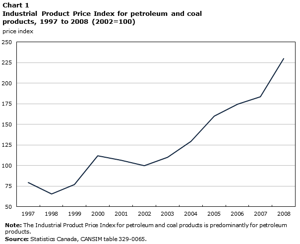
Description for Chart 1
| price index | |
|---|---|
| 1997 | 79.6 |
| 1998 | 65.5 |
| 1999 | 76.6 |
| 2000 | 111.7 |
| 2001 | 106.5 |
| 2002 | 100.0 |
| 2003 | 110.0 |
| 2004 | 129.4 |
| 2005 | 159.9 |
| 2006 | 174.2 |
| 2007 | 183.5 |
| 2008 | 230.2 |
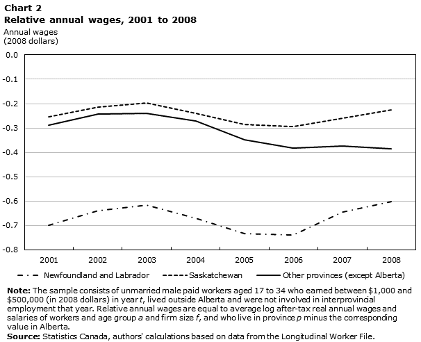
Description for Chart 2
| Newfoundland and Labrador | Saskatchewan | Other provinces (except Alberta) | |
|---|---|---|---|
| 2001 | -0.700 | -0.255 | -0.287 |
| 2002 | -0.638 | -0.214 | -0.243 |
| 2003 | -0.615 | -0.197 | -0.240 |
| 2004 | -0.671 | -0.241 | -0.270 |
| 2005 | -0.733 | -0.286 | -0.349 |
| 2006 | -0.740 | -0.293 | -0.382 |
| 2007 | -0.645 | -0.261 | -0.373 |
| 2008 | -0.601 | -0.227 | -0.386 |
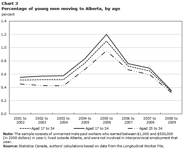
Description for Chart 3
| Aged 17 to 34 | Aged 17 to 24 | Aged 25 to 34 | |
|---|---|---|---|
| 2001 to 2002 | 0.513 | 0.554 | 0.452 |
| 2002 to 2003 | 0.514 | 0.571 | 0.430 |
| 2003 to 2004 | 0.516 | 0.577 | 0.426 |
| 2004 to 2005 | 0.768 | 0.831 | 0.674 |
| 2005 to 2006 | 1.100 | 1.199 | 0.952 |
| 2006 to 2007 | 0.723 | 0.760 | 0.667 |
| 2007 to 2008 | 0.650 | 0.689 | 0.593 |
| 2008 to 2009 | 0.343 | 0.356 | 0.325 |
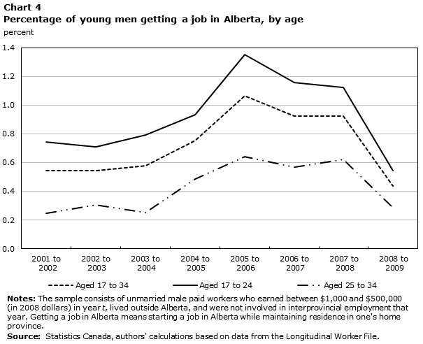
Description for Chart 4
| Aged 17 to 34 | Aged 17 to 24 | Aged 25 to 34 | |
|---|---|---|---|
| 2001 to 2002 | 0.542 | 0.743 | 0.247 |
| 2002 to 2003 | 0.546 | 0.708 | 0.307 |
| 2003 to 2004 | 0.576 | 0.793 | 0.253 |
| 2004 to 2005 | 0.754 | 0.934 | 0.486 |
| 2005 to 2006 | 1.065 | 1.351 | 0.640 |
| 2006 to 2007 | 0.922 | 1.159 | 0.570 |
| 2007 to 2008 | 0.922 | 1.124 | 0.623 |
| 2008 to 2009 | 0.438 | 0.542 | 0.284 |
5.2 Regression results
Table 4 shows regression results for the first sample; i.e., young men who earn at least $1,000 during the reference year. Regardless of the models considered, OLS estimates of are essentially equal to zero, thereby suggesting that workers do not respond to changes in the spatial earnings structure. Applying the 2SLS estimator to microdata leads to the rejection of this conclusion. For instance, Models 1 to 3 indicate that varies between -0.18 and -0.22. In other words, a 10% decline in annual wages relative to those paid in Alberta increases the probability of migrating to Alberta by between 1.8 percentage points (0.018) and 2.2 percentage points (0.022), from a baseline rate of 0.64%. 2SLS estimates based on grouped data are of similar magnitude and are about 20 times higher, in absolute value, than EWALD estimates.Note 26 As with Models 1 to 3, 2SLS estimates from Model 4 suggest that interprovincial mobility rises in response to widening cross-regional wage differences. However, these estimates are based on weaker first-stage regressions than those underlying Models 1 to 3 and, therefore, must be interpreted with caution.
Whether applied to microdata or grouped data, 2SLS estimates also generally indicate that a greater proportion of young men become interprovincial employees as cross-regional wage differences increase. Models 1 to 3 suggest that a 10% decline in wages relative to those paid in Alberta increases the probability of accepting a job in Alberta while maintaining residence in one’s home province by between 0.70 percentage points (0.007) and 1.0 percentage point (0.010), from a baseline rate of 0.72%.Note 27
Table 5 shows results for the second sample; i.e., young men who earn at least $15,000 during the reference year. For this sample, Models 1 to 3 yield 2SLS estimates of very similar to those obtained from the first sample, both in terms of migration and transitions into interprovincial employment.
The results presented so far are based on linear models and, thus, do not necessarily provide appropriate estimates of the average partial effect of annual wages on the binary outcomes considered. Table 6 deals with this issue and provides estimates of average partial effects of annual wages that are obtained after implementing the two-step method of Rivers and Vuong (1988). In the first sample, Models 1 to 3 indicate that a 10% decline in annual wages relative to those paid in Alberta increases the probability of migrating to Alberta by 0.7 percentage points to 0.8 percentage points. The corresponding increases in the likelihood of migrating vary between 0.7 percentage points and 0.9 percentage points in the second sample. Hence, for both samples, the average partial effects resulting from probit models with endogenous regressors are less than half those obtained from the linear models of Tables 4 and 5. This conclusion holds when average partial effects of annual wages on the likelihood of making a transition into interprovincial employment, as obtained from Table 6, are compared with those of Tables 4 and 5.
Tables 4 to 6 relate changes in migration rates to proportionate changes in relative annual wages. An important question is whether the findings from these tables hold when proportionate changes in migration rates are related to proportionate changes in relative wages. Table 7 answers this question for the first sample. It assesses whether the grouped data results of Table 4 hold when the dependent variable is modelled in logarithms, rather than in levels. Models 1 to 3 indicate that using logarithms yields somewhat lower wage elasticities, in absolute value, of the likelihood of migrating to Alberta.Note 28 For instance, these wage elasticities equal -31.3 when using logarithms in Model 3, compared with -33.1 when using levels. Table 7 also shows that the wage parameters for the likelihood of making a transition into interprovincial employment are, in Models 1 to 3, no longer statistically significant when the dependent variable is modelled in logarithms. Hence, results on the likelihood of moving to Alberta are robust to functional form issues, while results on the likelihood of making a transition into interprovincial employment are sensitive to functional form issues. This conclusion holds for the second sample (Table 8).
| Model 1 | Model 2 | Model 3 | Model 4 | |||||
|---|---|---|---|---|---|---|---|---|
| Outcome | Outcome | Outcome | Outcome | |||||
| Moving to Alberta | Getting a job in Alberta | Moving to Alberta | Getting a job in Alberta | Moving to Alberta | Getting a job in Alberta | Moving to Alberta | Getting a job in Alberta | |
| Mean of dependent variable | 0.0064 | 0.0072 | 0.0064 | 0.0072 | 0.0064 | 0.0072 | 0.0064 | 0.0072 |
| Estimate of (wage parameter) | ||||||||
| Microdata | ||||||||
| Ordinary least squares (OLS) | 0.000 | 0.000Note * | 0.000 | 0.000Note † | 0.000 | 0.000Note † | 0.000 | 0.000Note † |
| Two-stage least squares (2SLS) | -0.183Note *** | -0.081Note * | -0.217Note ** | -0.083Note * | -0.184Note *** | -0.070Note * | -0.336Note * | -0.149Note † |
| Grouped data | ||||||||
| Weighted least squares (EWALD) | -0.010Note *** | -0.003 | -0.007Note ** | 0.000 | -0.008Note ** | 0.000 | -0.002 | 0.004 |
| Two-stage least squares (2SLS) | -0.215Note *** | -0.098Note * | -0.256Note ** | -0.100Note † | -0.212Note *** | -0.083Note * | -0.433Note † | -0.198 |
| Number of clusters | 81 | 81 | 81 | 81 | 81 | 81 | 81 | 81 |
| Number of observations | ||||||||
| Microdata | 1,140,071 | 1,140,071 | 1,140,071 | 1,140,071 | 1,140,071 | 1,140,071 | 1,140,071 | 1,140,071 |
| Grouped data | 2,591 | 2,591 | 2,591 | 2,591 | 2,591 | 2,591 | 2,591 | 2,591 |
| Kleibergen-Paap Wald F-statistic (2SLS) | ||||||||
| Microdata | 19.1 | 19.1 | 12.9 | 12.9 | 17.8 | 17.8 | 6.2 | 6.2 |
| Grouped data | 14.9 | 14.9 | 9.2 | 9.2 | 13.2 | 13.2 | 3.3 | 3.3 |
Source: Statistics Canada, authors' calculations based on data from the Longitudinal Worker File. |
||||||||
| Model 1 | Model 2 | Model 3 | Model 4 | |||||
|---|---|---|---|---|---|---|---|---|
| Outcome | Outcome | Outcome | Outcome | |||||
| Moving to Alberta | Getting a job in Alberta | Moving to Alberta | Getting a job in Alberta | Moving to Alberta | Getting a job in Alberta | Moving to Alberta | Getting a job in Alberta | |
| Mean of dependent variable | 0.0058 | 0.0049 | 0.0058 | 0.0049 | 0.0058 | 0.0049 | 0.0058 | 0.0049 |
| Estimate of (wage parameter) | ||||||||
| Microdata | ||||||||
| Ordinary least squares (OLS) | 0.000 | 0.001Note † | 0.000 | 0.001Note † | -0.001 | 0.001Note † | 0.000 | 0.001Note † |
| Two-stage least squares (2SLS) | -0.239Note *** | -0.079Note ** | -0.249Note *** | -0.077Note * | -0.207Note *** | -0.064Note * | -0.507Note * | -0.169Note † |
| Grouped data | ||||||||
| Weighted least squares (EWALD) | -0.014Note ** | -0.003 | -0.008Note † | 0.000 | -0.010Note * | 0.000 | 0.008Note † | 0.008Note * |
| Two-stage least squares (2SLS) | -0.228Note *** | -0.078Note * | -0.238Note *** | -0.075Note * | -0.198Note *** | -0.063Note * | -0.514Note * | -0.176 |
| Number of clusters | 81 | 81 | 81 | 81 | 81 | 81 | 81 | 81 |
| Number of observations | ||||||||
| Microdata | 563,133 | 563,133 | 563,133 | 563,133 | 563,133 | 563,133 | 563,133 | 563,133 |
| Grouped data | 2,530 | 2,530 | 2,530 | 2,530 | 2,530 | 2,530 | 2,530 | 2,530 |
| Kleibergen-Paap Wald F-statistic (2SLS) | ||||||||
| Microdata | 48.3 | 48.3 | 38.4 | 38.4 | 52.4 | 52.4 | 8.2 | 8.2 |
| Grouped data | 42.7 | 42.7 | 33.6 | 33.6 | 45.6 | 45.6 | 6.7 | 6.7 |
Source: Statistics Canada, authors' calculations based on data from the Longitudinal Worker File. |
||||||||
| Model 1 | Model 2 | Model 3 | Model 4 | |||||
|---|---|---|---|---|---|---|---|---|
| Outcome | Outcome | Outcome | Outcome | |||||
| Moving to Alberta | Getting a job in Alberta | Moving to Alberta | Getting a job in Alberta | Moving to Alberta | Getting a job in Alberta | Moving to Alberta | Getting a job in Alberta | |
| First sample | ||||||||
| Mean of dependent variable | 0.0064 | 0.0072 | 0.0064 | 0.0072 | 0.0064 | 0.0072 | 0.0064 | 0.0072 |
| Relative annual wages | ||||||||
| Probit coefficient | -4.285Note *** | -1.965Note *** | -4.855Note *** | -1.578Note ** | -4.112Note *** | -1.338Note ** | -7.863Note *** | -3.613Note *** |
| Average partial effect | -0.072 | -0.036 | -0.082 | -0.029 | -0.069 | -0.024 | -0.132 | -0.066 |
| Number of clusters | 81 | 81 | 81 | 81 | 81 | 81 | 81 | 81 |
| Number of observations | 1,140,071 | 1,140,071 | 1,140,071 | 1,140,071 | 1,140,071 | 1,140,071 | 1,140,071 | 1,140,071 |
| Second sample | ||||||||
| Mean of dependent variable | 0.0058 | 0.0049 | 0.0058 | 0.0049 | 0.0058 | 0.0049 | 0.0058 | 0.0049 |
| Relative annual wages | ||||||||
| Probit coefficient | -5.787Note *** | -2.875Note *** | -5.673Note *** | -2.413Note *** | -4.720Note *** | -2.004Note *** | -12.290Note *** | -6.078Note *** |
| Average partial effect | -0.092 | -0.037 | -0.090 | -0.031 | -0.074 | -0.026 | -0.195 | -0.089 |
| Number of clusters | 81 | 81 | 81 | 81 | 81 | 81 | 81 | 81 |
| Number of observations | 563,133 | 563,133 | 563,133 | 563,133 | 563,133 | 563,133 | 563,133 | 563,133 |
Source: Statistics Canada, authors' calculations based on data from the Longitudinal Worker File. |
||||||||
| Model 1 | Model 2 | Model 3 | Model 4 | |||||
|---|---|---|---|---|---|---|---|---|
| Outcome | Outcome | Outcome | Outcome | |||||
| Moving to Alberta | Getting a job in Alberta | Moving to Alberta | Getting a job in Alberta | Moving to Alberta | Getting a job in Alberta | Moving to Alberta | Getting a job in Alberta | |
| Mean of dependent variable | 0.0064 | 0.0072 | 0.0064 | 0.0072 | 0.0064 | 0.0072 | 0.0064 | 0.0072 |
| Estimate of (wage parameter) | ||||||||
| Level–log | ||||||||
| Weighted least squares (EWALD) | -0.010Note *** | -0.003 | -0.007Note ** | 0.0 | -0.008Note ** | 0.0 | -0.002 | 0.004 |
| Two-stage least squares (2SLS) | -0.215Note *** | -0.098Note * | -0.256Note ** | -0.100Note † | -0.212Note *** | -0.083Note * | -0.433Note † | -0.198 |
| Log–log | ||||||||
| Weighted least squares (EWALD) | -0.943 | 0.921 | -1.160 | 1.263 | -1.276 | 1.333 | -1.448 | 1.687 |
| Two-stage least squares (2SLS) | -26.8Note ** | -3.0 | -37.8Note * | -0.9 | -31.3Note ** | -0.7 | -54.0Note † | -6.1 |
| Wage elasticities (2SLS) | ||||||||
| Level–log | -33.6 | -13.6 | -40.0 | -13.9 | -33.1 | -11.5 | -67.7 | -27.5 |
| Log–log | -26.8 | -3.0 | -37.8 | -0.9 | -31.3 | -0.7 | -54.0 | -6.1 |
| Number of clusters | 81 | 81 | 81 | 81 | 81 | 81 | 81 | 81 |
| Number of observations | 2,591 | 2,591 | 2,591 | 2,591 | 2,591 | 2,591 | 2,591 | 2,591 |
| Kleibergen-Paap Wald F-statistic (2SLS) | 14.9 | 14.9 | 9.2 | 9.2 | 13.2 | 13.2 | 3.3 | 3.3 |
Source: Statistics Canada, authors' calculations based on data from the Longitudinal Worker File. |
||||||||
| Model 1 | Model 2 | Model 3 | Model 4 | |||||
|---|---|---|---|---|---|---|---|---|
| Outcome | Outcome | Outcome | Outcome | |||||
| Moving to Alberta | Getting a job in Alberta | Moving to Alberta | Getting a job in Alberta | Moving to Alberta | Getting a job in Alberta | Moving to Alberta | Getting a job in Alberta | |
| Mean of dependent variable | 0.0058 | 0.0049 | 0.0058 | 0.0049 | 0.0058 | 0.0049 | 0.0058 | 0.0049 |
| Estimate of (wage parameter) | ||||||||
| Level–log | ||||||||
| Weighted least squares (EWALD) | -0.014Note ** | -0.003 | -0.008Note † | 0.000 | -0.010Note * | 0.000 | 0.008Note † | 0.008Note * |
| Two-stage least squares (2SLS) | -0.228Note *** | -0.078Note * | -0.238Note *** | -0.075Note * | -0.198Note *** | -0.063Note * | -0.514Note * | -0.176 |
| Log–log | ||||||||
| Weighted least squares (EWALD) | -5.840Note † | 0.788 | -5.126 | 1.055 | -5.028 | 1.229 | -1.855 | 1.457 |
| Two-stage least squares (2SLS) | -31.3Note *** | -8.7 | -32.7Note ** | -9.2 | -27.2Note ** | -7.6 | -70.4Note * | -19.5 |
| Wage elasticities (2SLS) | ||||||||
| Level–log | -39.3 | -15.9 | -41.0 | -15.3 | -34.1 | -12.9 | -88.6 | -35.9 |
| Log–log | -31.3 | -8.7 | -32.7 | -9.2 | -27.2 | -7.6 | -70.4 | -19.5 |
| Number of clusters | 81 | 81 | 81 | 81 | 81 | 81 | 81 | 81 |
| Number of observations | 2,530 | 2,530 | 2,530 | 2,530 | 2,530 | 2,530 | 2,530 | 2,530 |
| Kleibergen-Paap Wald F-statistic (2SLS) | 42.7 | 42.7 | 33.6 | 33.6 | 45.6 | 45.6 | 6.7 | 6.7 |
Source: Statistics Canada, authors' calculations based on data from the Longitudinal Worker File. |
||||||||
5.3 Implications for job vacancies
The degree to which worker movements to Alberta reduced job vacancies during the 2001-to-2008 period depends on the increase in aggregate annual work hours that resulted from these movements. If all young men who moved to Alberta worked full-time on a full-year basis in their home province prior to migrating and did not increase their work hours afterwards, and if their departure from their home province created a job vacancy that remained unfilled, then migration to Alberta would reduce job vacancies in that province while increasing vacancies elsewhere, leaving unchanged the total number of vacant positions in Canada. Conversely, if migrants left jobs that were subsequently filled by unemployed individuals in their home province, then migration to Alberta would reduce the aggregate number of job vacancies in Canada by an amount equal to the number of migrants. Thus, the increase in the expected number of migrants associated with a given increase in Alberta’s relative annual wages provides an upper bound for the degree to which changes in the regional wage structure reduced job vacancies in Canada during the observation period.
From 2001 to 2005, real average annual wages and salaries earned by unmarried men (of a given age and employed in a given firm-size category and a given province) relative to those of their counterparts in Alberta fell by about 6%, from -0.29 in 2001 to -0.35 in 2005 (Table 3-1). Multiplying the average partial effect obtained from probit Model 3 using the first sample (-0.069, see Table 6)―the preferred specification―by -0.06 yields a predicted increase in migration rate of 0.4 percentage points. Note 29,Note 30 Multiplying this increase (0.004) by 10 times the average sample size () yields the predicted increase in the number of young male migrants; i.e., 5,900. Since private-sector locations operating in Alberta had between 37,000 and 48,000 job vacancies from 2001 to 2005 (Table 9), the estimated increase in the number of young male migrants represents between 12% and 16% of the number of job vacancies observed in Alberta during the 2001-to-2005 period.
This conclusion is strengthened by computing the estimated increase in the number of young male migrants that results from a decline of 9% (rather than 6%) in relative annual wages, which is the decline observed from 2001 to 2006 (Table 3-1). In that case, the estimated increase in the number of young male migrants represents between 18% and 24% of the number of job vacancies observed in Alberta during the 2001-to-2005 period. Regardless of the scenario considered, these numbers suggest that increased annual wages paid in Alberta induced flows of young male workers that represent a significant proportion of the job vacancies observed in that province.
| Year and data source | Job vacancies |
|---|---|
| number | |
| 2001 Workplace and Employee Survey | 37,256 |
| 2003 Workplace and Employee Survey | 32,631 |
| 2005 Workplace and Employee Survey | 48,143 |
| 2011 Business Payrolls Survey | 43,880 |
| 2012 Business Payrolls Survey | 60,100 |
| 2013 Business Payrolls Survey | 48,508 |
| 2014 Business Payrolls Survey | 48,283 |
|
Notes: Job vacancies in businesses operating in all industries except farming, fishing, hunting, and public administration. No data on job vacancies are available for the years 2006 to 2010. Source: Statistics Canada, authors' calculations based on data from the Workplace and Employee Survey and CANSIM table 284-0001. |
|
6 Concluding remarks
Quantifying the degree to which the geographic mobility of workers responds to spatial movements in annual wages is a difficult task that requires both the use of large datasets and the identification of exogenous variation in cross-regional wage movements. This article tackles these challenges by using mobility information from a large administrative dataset and identifying the exogenous variation in cross-regional earnings movements plausibly induced by substantial increases in oil prices observed during the 2000s.
The empirical strategy of the study takes advantage of the fact that the oil boom of the 2000s generated a natural experiment in which annual earnings grew much faster in the three oil-producing provinces of Canada than in the other provinces. These spatial movements in the earnings structure increased the incentives for individuals to move to the biggest oil-producing province, Alberta, or to accept job offers in that province while maintaining residence in their home province.
The main finding of the study is that even though migration to Alberta and transitions into interprovincial employment in that province were relatively rare events for young unmarried male paid workers during the 2000s—affecting less than 1% of them on an annual basis—the likelihood of these events occurring varied significantly in response to spatial movements in the earnings structure. The results of this study indicate that faster growth in real annual wages and salaries in Alberta, compared with other provinces, substantially increased migration to Alberta. The resulting worker inflows represented a significant fraction of the job vacancies observed in that province during the 2000s. There is also evidence that changes in the regional wage structure fostered transitions into interprovincial employment in Alberta. Whether the magnitude of these responses is optimal, and to what degree these responses were constrained by barriers to mobility, are questions left for further research.
7 Appendix tables
| Microdata | Grouped data | |||
|---|---|---|---|---|
| Outcome | Outcome | |||
| Moving to Alberta | Getting a job in Alberta | Moving to Alberta | Getting a job in Alberta | |
| estimate | ||||
| Mean of dependent variable | 0.0064 | 0.0072 | 0.0064 | 0.0072 |
| Relative annual earnings | -0.183Note *** | -0.081Note ** | -0.215Note *** | -0.098Note * |
| Attending a postsecondary institution in year t | -0.046Note *** | -0.019Note * | -0.059Note * | -0.002 |
| Laid off in year t | -0.021Note * | -0.005 | -0.090Note * | -0.047Note † |
| Laid off in year | -0.014Note ** | -0.001 | -0.042Note † | -0.010 |
| Paying union dues in year t | 0.010Note ** | 0.005Note ** | 0.001 | -0.001 |
| Having a positive pension adjustment in year t | 0.076Note *** | 0.033Note * | 0.132Note *** | 0.062Note * |
| RRSP contributions in year t ($'000) | 0.013Note *** | 0.006Note * | 0.017Note ** | 0.009Note * |
| Relative unemployment rates | 0.000 | 0.000 | 0.000 | 0.000 |
| Relative rates of involuntary part-time employment | -0.001Note † | -0.001Note * | -0.001Note * | -0.001Note * |
| Relative minimum wages | -0.035Note † | -0.001 | -0.038Note † | -0.002 |
| Year effects | ||||
| 2002 | 0.010Note *** | 0.004Note * | 0.012Note *** | 0.005Note * |
| 2003 | 0.012Note *** | 0.005Note * | 0.013Note *** | 0.005Note † |
| 2004 | 0.010Note *** | 0.004Note * | 0.010Note *** | 0.004Note * |
| 2005 | -0.003 | 0.001 | -0.005 | -0.001 |
| 2006 | -0.014Note *** | -0.003 | -0.019Note *** | -0.005 |
| 2007 | -0.014Note *** | -0.003 | -0.018Note *** | -0.005 |
| 2008 | -0.020Note *** | -0.008Note ** | -0.024Note *** | -0.010 |
| value | ||||
| Kleibergen-Paap Wald F-statistic (2SLS) | 19.1 | 19.1 | 14.9 | 14.9 |
| number | ||||
| Clusters | 81 | 81 | 81 | 81 |
| Groups | Note ...: not applicable | Note ...: not applicable | 324 | 324 |
| Observations | 1,140,071 | 1,140,071 | 2,591 | 2,591 |
... not applicable
Source: Statistics Canada, authors’ calculations based on data from the Longitudinal Worker File. |
||||
| Microdata | Grouped data | |||
|---|---|---|---|---|
| Outcome | Outcome | |||
| Moving to Alberta | Getting a job in Alberta | Moving to Alberta | Getting a job in Alberta | |
| estimate | ||||
| Mean of dependent variable | 0.0064 | 0.0072 | 0.0064 | 0.0072 |
| Relative annual earnings | -0.184Note *** | -0.070Note * | -0.212Note *** | -0.083Note * |
| Relative annual rent | 0.045 | -0.003 | 0.046 | -0.004 |
| Attending a postsecondary institution in year t | -0.047Note *** | -0.016Note * | -0.057Note * | -0.016 |
| Laid off in year t | -0.022Note * | -0.003 | -0.082Note * | -0.040Note † |
| Laid off in year | -0.014Note * | 0.000 | -0.042Note † | -0.007 |
| Paying union dues in year t | 0.010Note ** | 0.004Note * | -0.003 | -0.003 |
| Having a positive pension adjustment in year t | 0.076Note *** | 0.028Note * | 0.118Note ** | 0.053Note * |
| RRSP contributions in year t ($'000) | 0.013Note *** | 0.005Note * | 0.017Note * | 0.008Note † |
| Relative unemployment rates | 0.000 | 0.000 | 0.000 | 0.000 |
| Relative rates of involuntary part-time employment | -0.001Note † | -0.001Note * | -0.001Note † | -0.001Note * |
| Relative minimum wages | -0.033 | 0.006 | -0.034 | 0.006 |
| Year effects | ||||
| 2002 | 0.007Note *** | 0.003Note * | 0.008Note *** | 0.003Note † |
| 2003 | 0.008Note * | 0.002 | 0.008Note * | 0.002 |
| 2004 | 0.003Note * | 0.002Note † | 0.003 | 0.001 |
| 2005 | -0.007Note † | 0.000 | -0.010Note * | -0.002 |
| 2006 | -0.022Note *** | -0.005 | -0.027Note ** | -0.008 |
| 2007 | -0.021Note *** | -0.007Note * | -0.026Note *** | -0.011Note * |
| 2008 | -0.027Note *** | -0.013Note *** | -0.032Note *** | -0.016Note ** |
| value | ||||
| Kleibergen-Paap Wald F-statistic (2SLS) | 17.8 | 17.8 | 13.2 | 13.2 |
| number | ||||
| Clusters | 81 | 81 | 81 | 81 |
| Groups | Note ...: not applicable | Note ...: not applicable | 324 | 324 |
| Observations | 1,140,071 | 1,140,071 | 2,591 | 2,591 |
... not applicable
Source: Statistics Canada, authors’ calculations based on data from the Longitudinal Worker File. |
||||
| Model 1 | Model 2 | Model 3 | Model 4 | |||||
|---|---|---|---|---|---|---|---|---|
| Outcome | Outcome | Outcome | Outcome | |||||
| Moving to Alberta | Getting a job in Alberta | Moving to Alberta | Getting a job in Alberta | Moving to Alberta | Getting a job in Alberta | Moving to Alberta | Getting a job in Alberta | |
| Mean of dependent variable | 0.0069 | 0.0092 | 0.0069 | 0.0092 | 0.0069 | 0.0092 | 0.0069 | 0.0092 |
| Estimate of (wage parameter) | ||||||||
| Microdata | ||||||||
| Ordinary least squares (OLS) | 0.001Note ** | 0.000 | 0.001Note ** | 0.000 | 0.001Note ** | 0.000 | 0.001Note ** | 0.000 |
| Two-stage least squares (2SLS) | -0.217Note *** | -0.127Note ** | -0.291Note ** | -0.149Note * | -0.240Note ** | -0.123Note ** | -0.441Note * | -0.258Note † |
| Grouped data | ||||||||
| Weighted least squares (EWALD) | -0.018Note *** | -0.009Note † | -0.015Note *** | -0.004 | -0.016Note *** | -0.005 | -0.009Note * | 0.002 |
| Two-stage least squares (2SLS) | -0.277Note *** | -0.169Note ** | -0.365Note * | -0.197Note * | -0.289Note ** | -0.156Note * | -0.611 | -0.374 |
| Number of clusters | 36 | 36 | 36 | 36 | 36 | 36 | 36 | 36 |
| Number of observations | ||||||||
| Microdata | 679,888 | 679,888 | 679,888 | 679,888 | 679,888 | 679,888 | 679,888 | 679,888 |
| Grouped data | 1,152 | 1,152 | 1,152 | 1,152 | 1,152 | 1,152 | 1,152 | 1,152 |
| Kleibergen-Paap Wald F-statistic (2SLS) | ||||||||
| Micro data | 12.9 | 12.9 | 7.3 | 7.3 | 10.5 | 10.5 | 4.0 | 4.0 |
| Grouped data | 9.1 | 9.1 | 4.9 | 4.9 | 7.5 | 7.5 | 1.9 | 1.9 |
Source: Statistics Canada, authors' calculations based on data from the Longitudinal Worker File. |
||||||||
| Model 1 | Model 2 | Model 3 | Model 4 | |||||
|---|---|---|---|---|---|---|---|---|
| Outcome | Outcome | Outcome | Outcome | |||||
| Moving to Alberta | Getting a job in Alberta | Moving to Alberta | Getting a job in Alberta | Moving to Alberta | Getting a job in Alberta | Moving to Alberta | Getting a job in Alberta | |
| Mean of dependent variable | 0.0056 | 0.0043 | 0.0056 | 0.0043 | 0.0056 | 0.0043 | 0.0056 | 0.0043 |
| Estimate of (wage parameter) | ||||||||
| Microdata | ||||||||
| Ordinary least squares (OLS) | -0.001Note *** | -0.001Note *** | -0.001Note *** | -0.001Note *** | -0.001Note *** | -0.001Note *** | -0.001Note *** | -0.001Note *** |
| Two-stage least squares (2SLS) | -0.135Note ** | -0.004 | -0.140Note * | 0.008 | -0.120Note * | 0.007 | -0.215 | -0.006 |
| Grouped data | ||||||||
| Weighted least squares (EWALD) | -0.003 | 0.000 | -0.001 | 0.001 | -0.001 | 0.002 | 0.003 | 0.004Note † |
| Two-stage least squares (2SLS) | -0.141Note * | -0.006 | -0.147Note * | 0.010 | -0.125Note * | 0.008 | -0.253 | -0.011 |
| Number of clusters | 45 | 45 | 45 | 45 | 45 | 45 | 45 | 45 |
| Number of observations | ||||||||
| Microdata | 460,183 | 460,183 | 460,183 | 460,183 | 460,183 | 460,183 | 460,183 | 460,183 |
| Grouped data | 1,439 | 1,439 | 1,439 | 1,439 | 1,439 | 1,439 | 1,439 | 1,439 |
| Kleibergen-Paap Wald F-statistic (2SLS) | ||||||||
| Microdata | 10.7 | 10.7 | 8.4 | 8.4 | 11.5 | 11.5 | 4.2 | 4.2 |
| Grouped data | 8.7 | 8.7 | 6.1 | 6.1 | 8.6 | 8.6 | 2.5 | 2.5 |
Source: Statistics Canada, authors' calculations based on data from the Longitudinal Worker File. |
||||||||
References
Abowd, J., F. Kramarz, and D. Margolis. 1999. “High wage workers and high wage firms.” Econometrica 67 (2): 251–333.
Amirault, D., D. de Munnik, and S. Miller. 2012. What Drags and Drives Mobility: Explaining Canada’s Aggregate Migration Patterns. Bank of Canada Working Paper no. 2012-28. Ottawa: Bank of Canada.
Bernard, A., R. Finnie, and B. St-Jean. 2008. “Interprovincial mobility and earnings.” Perspectives on Labour and Income 20 (4): 15–25. Statistics Canada Catalogue no. 75-001-X.
Coulombe, S. 2006. “Internal migration, asymmetric shocks, and interprovincial economic adjustments in Canada.” International Regional Science Review 29 (2): 199–223.
Dahl, G.B. 2002. “Mobility and the return to education: Testing a Roy model with multiple markets.” Econometrica 70 (6): 2367–2420.
Day, K.M. 1992. “Interprovincial migration and local public goods.” Canadian Journal of Economics 25 (1): 123–144.
Ferrer, A., and S. Lluis. 2008. “Should workers care about firm size?” Industrial Labor Relations Review 62 (1): 104–125.
Finnie, R. 2004. “Who moves? A logit model analysis of inter-provincial migration in Canada.” Applied Economics 36: 1759–1779.
Greenwood, M.J. 1997. “Internal migration in developed countries.” In Handbook of Population and Family Economics, ed. M.R. Rozenwig and O. Stark, volume 1, part B, chapter 12, p. 647–720. New York: Elsevier Science, North Holland.
Harris, J.R., and M.P. Todaro. 1970. “Unemployment and development: A two-sector analysis.” American Economic Review 60 (1): 126–142.
Kennan, J., and J.R. Walker. 2011. “The effect of expected income on individual migration decisions.” Econometrica 79 (1): 211–251.
Laporte, C., Y. Lu, and G. Schellenberg. 2013. Inter-provincial Employees in Alberta. Analytical Studies Branch Research Paper Series, no. 350. Statistics Canada Catalogue no. 11F0019M. Ottawa: Statistics Canada.
Lewbel, A., Y. Dong, and T.T. Yang. 2012. “Comparing features of convenient estimators for binary choice models with endogenous regressors.” Canadian Journal of Economics 45 (3): 809–829.
Lowry, I.S. 1966. Migration and Metropolitan Growth: Two Analytical Models. San Francisco: Chandler.
Milligan, K. 2012. Canadian Tax and Credit Simulator. Database, software and documentation, Version 2012-1.
Molloy, R., C.L. Smith, and A. Wozniak. 2011. “Internal migration in the United States.” Journal of Economic Perspectives 25 (3): 173–196.
Morissette, R. 1993. “Canadian jobs and firm size: Do smaller firms pay less?” Canadian Journal of Economics 26 (1): 159–174.
Morissette, R., P.C.W. Chan, and Y. Lu. 2015. “Wages, youth employment, and school enrollment: Recent evidence from increases in world oil prices.” Journal of Human Resources 50 (1): 222–253.
Ravenstein, E.G. 1885. “The laws of migration.” Journal of the Royal Statistical Society of London 48 (2): 167–235.
Rivers, D., and Q.H. Vuong. 1988. “Limited information estimators and exogeneity tests for simultaneous probit models.” Journal of Econometrics 39 (3): 347–366.
Stock, J., and M. Watson. 2011. Introduction to Econometrics. 3rd edition. Boston: Addison-Wesley.
Wooldridge, J.M. 2010. Econometric Analysis of Cross Section and Panel Data. 2nd edition. Cambridge: MIT Press.
- Date modified: