
Analytical Studies: Methods and References
Measuring the Correlation Between COVID-19 Restrictions and Economic Activity
Skip to text
Text begins
Acknowledgements
The authors would like to express their thanks to Danny Leung, Claudia Sanmartin, Guy Gellatly and Yvan Clermont for their support and guidance during the course of the project. They would also like to thank Calista Cheung and Charles Breton for their comments and feedback.
Abstract
This paper develops COVID-19 restrictions indexes for all Canadian provinces and territories. Indexes are produced daily and illustrate the overall level of restrictions and differences in restrictions on the vaccinated and unvaccinated portions of the population. The indexes show that restrictions in Ontario and Quebec were more stringent and remained in force for longer and at higher levels than in British Columbia and Alberta. They also illustrate the more stringent restrictions faced by the unvaccinated population as vaccination campaigns unfolded. When the daily indexes are converted to a monthly frequency, they show that after the first wave of COVID-19, increasing the severity of restrictions slows growth in economic activity as long as the severity of these restrictions remains below a threshold value. After the threshold value is reached, tighter restrictions are associated with declines in economic activity.
The indexes build on the Oxford University Stringency Index by increasing the granularity of categories, adding additional variables, and providing a method for reporting on and weighting together vaccinated and unvaccinated populations. The indexes reported herein encompass a broad range of public health restrictions on personal activity (e.g., gathering sizes), childcare and education, and business activity (e.g., non-essential retail closures).
1 Introduction
The COVID-19 pandemic ushered in unprecedented peacetime restrictions on economic and social activity around the world. Restrictions on gathering sizes, recreation, travel and business activities were enacted across Canada and other countries in an effort to limit personal contact and slow the spread of the disease. In Canada, these restrictions often took different forms between the provinces and territories and over time.
Since restrictions were enacted differently over time and across jurisdictions, it is not straightforward to make comparisons or to enumerate their effects. Nevertheless, the restrictions had important impacts on the economy and society. There were also different levels of stringency to the restrictions across the provinces and territories. As a result, a measure of when restrictions were enacted, how strong they were and how long they lasted is considerably valuable, even if the measurement is not perfect.
Therefore, to facilitate comparisons, a COVID-19 restrictions index was developed to measure the severity of restrictions in the provinces and territories. The index builds on the Stringency Index developed by Oxford University [1] in a similar manner to the ones produced by the Bank of Canada [2] and the Institute for Research on Public Policy (IRPP) [3]. Because the Bank of Canada and IRPP indexes also use the Oxford index as a starting point, there are similarities between those and the ones reported here. However, the indexes reported here have four adjustments compared to the Oxford indexes, and there is some overlap with the Bank of Canada and IRPP indexes. Adjustments for bin sizes, the restrictions included, and the treatment of the vaccinated and unvaccinated populations are designed to produce more “Canada-centric” values. Adjustments for exponential scaling are designed to accentuate movements across pandemic waves. As a result, the indexes reported here provide more information than other current indexes on how restrictions were employed during the pandemic.Note
To produce a more “Canada-centric” index, the bins used in the Oxford index were first modified based on the thresholds in the restrictions that were used in the provinces and territories. For example, rather than a single variable to capture gathering size limits, separate categories were used to distinguish between indoor and outdoor gatherings. In addition, smaller bin sizes were used. For example, for indoor gatherings, bins that correspond to “prohibited, family only or 5 or less,” “10 or less”, “ 25 or less”, “50 or less”, “100 or less”, “250 or less” and “no restrictions” were implemented to reflect common restrictions used across the provinces rather than the larger “10 people or less”, “11 to 100” and “101 to 1000”, “1001 or more”, “no restrictions” buckets used in the Oxford index.
Second, additional variables were added to better reflect the restrictions enacted in Canada. These variables correspond to business restrictions (e.g., restaurant capacity limits for dining in versus take-out only) or business types (e.g., gyms, hair salons or non-essential retail) that were forced to close during certain periods or were instructed to implement capacity restraints. While a large number of restriction variables were available to choose from, considerable effort was taken to ensure that the additional variables were common (or as common as possible) across the provinces and territories.
Third, vaccination status within the vaccine-eligible Canadian population is taken into account.Note In early September 2021, the provinces introduced restrictions based on vaccination status. As a result, each restriction type for the indexes reported is split by vaccination status. This allows these indexes to not only present information on the stringency of restrictions according to vaccination status for those eligible for the vaccine, but also weight the vaccination statuses together to provide an overall level of restriction stringency. For instance, gyms were allowed to open only for vaccinated people, with restrictions for masks and physical distancing in place. Meanwhile, unvaccinated people were not allowed to enter gym facilities. In this case, the restriction for gyms is recorded as 1 (fully open with health measures in place) for the vaccinated population and 3 (closed) for the unvaccinated population. These are reported as separate index values depending on vaccine status, and allow for a gym score that is calculated based on the weighted sum of the vaccinated and unvaccinated populations of each province.
Fourth, the bin values were scaled so that the effect of imposing mild restrictions is smaller than when a more severe restriction is imposed. This means that moving from lower to higher levels of restrictions is assumed to have an increasingly stronger effect. For example, the move from having no restrictions to wearing a mask being recommended while in school leads to a smaller increase in the restrictions index than the change from partial online learning to schools closing.
The results from the indexes show that Ontario and Quebec tended to implement stronger restrictions for longer periods of time, while Alberta and British Columbia tended to have comparatively modest restriction levels. Moreover, restrictions tended to be common within regions—particularly for New Brunswick, Nova Scotia, Prince Edward Island, and Newfoundland and Labrador, which all participated in an Atlantic bubble. Once vaccination became more widespread, a noticeable difference emerged between the restrictions placed on the vaccinated and unvaccinated populations. However, this difference disappeared in the winter of 2021/2022 as COVID-19 cases increased rapidly. Across the types of restrictions in the index, restrictions on personal activities, such as limited gathering sizes or restrictions on internal movement, tended to be common and were implemented often. Restrictions on business activity were the second most common and included closing nonessential retail businesses, closing gyms and restrictions on in-person dining. The closure of schools and daycares became rarer after the first wave of COVID-19.
The index can also be used to help understand how the pandemic affected other types of activity. When employment, retail sales and the number of active firms are examined using pooled data from the second and third waves of COVID-19, statistical models show a negative impact on the growth in economic variables from increasing restrictions. Moreover, when the level of restrictions is low, increasing the restrictions acts to slow down growth. As restrictions become more stringent, they pass a threshold (the value of 41 on the indexes), and the effect of tightening restrictions then has a larger impact on economic variables that can correspond with outright declines.
At a value of 41, restrictions tend to go from being an inconvenience (e.g., wear a mask and gather only in smaller groups) to being a burden (e.g., in-person schooling is cancelled, nonessential retail and personal services are closed, or stay-at-home orders are issued). The value of 41, therefore, represents a point at which restrictions tend to become more binding for personal and business activities, and thus represents a level above which increases in restrictions can lead to more noticeable changes in activity. Numerically, the models suggest that below the threshold value, growth of 10 percentage points in the restrictions index is associated with retail sales growth slowing by about 0.4 percentage points, with employment growth slowing by 0.2 percentage points, and with the growth rate in the number of active firms slowing by 0.1 percentage points. Once restriction levels surpass the threshold value, growth of 10 percentage points in the restrictions index is associated retail sales growth slowing by 1.0 percentage points, with employment growth slowing by 0.6 percentage points, but the response of the active firm growth rate is little changed at a reduction of 0.1 percentage points.
The remainder of this paper is structured as follows: Section 2 describes the measurement of the index, including the variables and the index aggregation formula. Section 3 presents the indexes as well as their correlation with and probable impact on retail sales, employment and the number of active businesses. Section 4 concludes.
2 Index measurement
The objective of the indexes is to provide a measure of the combined strength of the COVID-19-related restrictions implemented over time by provincial and territorial governments throughout the country. The indexes are compiled daily from provincial and territorial public health websites, news reports and government publications. They are meant to identify similar types of restrictions regardless of their labels (e.g., red zone) or the jurisdiction in which they are imposed.
The approach to index construction necessitates a trade-off between measurement accuracy and comparability. Not all provinces and territories enacted the same types of restrictions in the same way and at the same time. This makes it challenging to define common categories to classify specific restrictions. For example, interprovincial and intraprovincial travel restrictions are grouped with curfews. These types of restrictions were used differently, at different times and in different places, but needed to be coded using the same schema to produce comparability over time and across geographies. Consequently, the provincial and territorial indexes are generally comparable over time and across geographies, but can obscure more nuanced differences in the nature of individual restrictions across jurisdictions.
2.1 Index construction
The restrictions indexes measure the severity of containment policies related to COVID-19. For each province or territory, the restrictions index is the average of 15 policy-specific indexes where the policy-specific indexes are normalized values of corresponding policy indicators. Eight of the indexes are derived (with some modifications) from the variables in the Oxford Stringency Index (Table 1). Seven additional variables are added to the index to better reflect the policy stance of Canadian jurisdictions.
| Sub-index | Identifier | Description | Source |
|---|---|---|---|
| I1 | C1—School closing | Record closings of schools and universities. | ... |
| I2 | C2—Workplace closing | Record closings of workplaces. | Oxford, with additions or changes when deemed necessary |
| I3 | C3—Cancel public events | Record cancelling of public events. | ... |
| I4 | C5—Close public transport | Record closings of public transportation. | ... |
| I5 | C6—Stay at home requirements | Record orders to “shelter-in-place” and otherwise confine to the home. | ... |
| I6 | C7—Restrictions on internal movement | Record restrictions on internal movement within or between cities or regions. | ... |
| I7 | C8—International travel controls | Record restrictions on international travel. Note: This records policy for foreign travellers, not for citizens. |
... |
| I8 | H1—Public information campaigns | Record the presence of public information campaigns | ... |
| I9 | C9—Restrictions on restaurants for in-person dining | Record restrictions on in-person dining at restaurants. Note: This records policy does not include limitations on liquor service at restaurants or what time a restaurant has to close. |
Statistics Canada |
| I10 | C10—Restrictions on gathering indoors | Record limits on indoor personal gathering. Note: This records policy does not include personal gatherings such as weddings and funerals. |
... |
| I11 | C11—Restrictions on gathering outdoors | Record limits on outdoor personal gathering. | ... |
| I12 | C12—Hair salons and barbershop closures | Record restrictions on hair salons and barbershops. | ... |
| I13 | C13—Daycare closing | Record closings of daycares or limiting them to the children of essential workers. | ... |
| I14 | C14—Restrictions on non-essential retail businesses | Record restrictions on non-essential retail businesses. | ... |
| I15 | C15—Gyms closing | Record closing fitness centres or gyms. | ... |
|
... not applicable Source: Statistics Canada. |
|||
Because most containment measures are issued by governments at the provincial, territorial or health region level, the restrictions index mostly reflects differences in provincial or territorial restriction policies over time. The main exception is the international travel restrictions indicator (C8), which captures federal policies imposed uniformly across the country. Although this variable does not add any additional information when comparing the index across provinces, it does reflect the stringency of travel restrictions that can correlate with variables such as border crossings, and can provide an indication of the performance of the Canadian economy, mental health, the ability of families to visit and societal stress.
2.2 Index construction
The methodology of these indexes follows a modified version of the methodology used to construct the Oxford Stringency Index.
For each indicator listed in Table 1, a value is assigned using an ordinal scale ranging from least restrictive (value of 0) to most restrictive (values of 2 to 6, depending on the indicator). The values are recorded based on a consistent set of coding requirements.Note These requirements were determined based on values taken from Oxford and the joint evaluations of the project team, and they reflect consensus decisions and revisions that arose as coding progressed. In addition to the ordinal scales, each policy indicator has a geographic scalar indicating whether the policy is general (1) or targeted to a particular health region (0) within a province.
Once restrictions are differentiated by vaccine status, the restriction values are divided between the vaccinated and unvaccinated populations, and recorded based on the coding requirements for the separate restrictions announced by the province. The restrictions for the vaccinated and unvaccinated populations can then be reported separately. Additionally, the value for the total population can be constructed as the weighted sum of the vaccinated and unvaccinated variables. The weights are based on the vaccinated and unvaccinated proportions of the population eligible for vaccination.
To produce an index for a specific indicator, the ordinal values are scaled to fall between 0 and 100 using the largest ordinal value. In the Oxford approach, the changes between levels of restrictions are equal so that the coding sequence (0,1, 2, 3, 4) becomes (0.25, 50, 75, 100), such that a unit change in the severity of the index corresponds to an increase of 25 percentage points.
However, in terms of their effects on the economy, mental health or societal stress, it is likely that stronger restrictions have a larger impact. To incorporate the increasing impact of progressively tighter restrictions, the present indicator-specific indexes are calculated after squaring the ordinal values. This means that the ordinal values (0, 1, 2, 3, 4) are rescaled (0, 1, 4, 9, 16) before being normalized (0, 6.25, 25.00, 56.25, 100.00). As a consequence, changes in the indexes are accentuated, particularly for periods when tighter restrictions come into effect.
Formally, the indicator-specific indexes are calculated as follows:
where is the recorded policy value on the ordinal scale. is the recorded binary flag for indicator and takes a value of 1 if the restriction is general to the province or territory and a value of 0 if the restriction is targeted to a specific city or health region. is a binary variable and takes a value of 1 if that indicator has a flag variable and takes a value of 0 if the indicator does not have a flag variable. is the maximum ordinal value of the indicator.
When policy is different for the vaccinated and unvaccinated populations, the indicator-specific indexes are calculated as follows:
where is the vaccination rate for fully vaccinated people as a share of the eligible population, is the recorded policy value for the vaccinated population, and is the recorded policy value for the unvaccinated population.
After calculating normalized index values for each indicator, the COVID-19 restrictions index for a province at time t is calculated by taking the average of the 15 policy-specific indexes:
2.3 Methodology comparison
To produce an index that is representative of the types and combinations of restrictions imposed in Canada, the Oxford variables are taken as a starting point. The Oxford restrictions are then adjusted or augmented where necessary, and the index formula is modified. The changes are implemented to create indexes that are more suited for making comparisons across Canadian jurisdictions than across countries.
The first difference between this index and the Oxford index pertains to the bins used to construct the indexes. For the variables that align with those from the Oxford index, the bins are modified as necessary to better reflect the Canadian experience. To allow for more granularity, the Oxford restriction on private gatherings (C4) is replaced by C10: restrictions on gathering indoors and C11: restrictions on gathering outdoors. When this was done smaller bin sizes were used. For example, for indoor gatherings, bins that correspond to “prohibited, family only or 5 or less,” “10 or less”, “ 25 or less”, “50 or less”, “100 or less”, “250 or less” and “no restrictions” were implemented to reflect common restrictions used across the provinces rather than the larger “10 people or less”, “11 to 100” and “101 to 1000”, “1001 or more”, “no restrictions” buckets used in the Oxford index.
Second, to increase the sensitivity of the indexes to Canada’s experience, the following seven additional variables are added:
- C9—restrictions on restaurants for in-person dining
- C10—restrictions on gathering indoors
- C11—restrictions on gathering outdoors
- C12—hair salons and barbershop closures
- C13—daycare closing
- C14—restrictions on non-essential retail businesses
- C15—gyms closing.
The additional variables capture areas where more granularity was warranted (C10 and C11), where Canadian authorities often targeted restrictions (C9, C12, C14 and C15), or where restrictions appear to have been particularly binding for home and work life (C13). The additional variables are not a complete list of all restriction types, and neither are the number of categories reflective of all situations. However, as a group, these categories capture the majority of restrictions used by policymakers across Canada and represent the types of public health measures enacted over the course of the pandemic.
Lastly, the index formula is adjusted so that the marginal change in the index becomes progressively larger as restrictions tighten. In effect, this accentuates periods of tight restrictions and increases the cyclicality of the indexes relative to those reported by Oxford.
Not all provinces and territories enacted the same set of restrictions. As a result, it is necessary to interpret the results with caution, since an index may increase if (1) more types of restrictions are put in place or (2) existing restrictions are tightened. One jurisdiction may implement a smaller set of tighter, more stringent restrictions, while another may implement a larger set of less stringent restrictions. Both situations could yield an identical index value. Therefore the index provides a method for comparing restriction levels across the jurisdictions, but in cases where levels are similar for two jurisdictions, it can be difficult to state which set of restrictions is stronger when using the index values in isolation.
In cases where more stringent policy responses apply only to specific health regions within a province or territory rather than to the whole province, the indicator is reduced by half a point from the ordinal value, regardless of the size of the health region relative to the provincial population.
The Bank of Canada and the IRPP also produce restriction indexes that incorporate elements of the Oxford indexes. The Bank of Canada indexes have some overlap with the indexes produced here as both set of indexes use a number of the same Oxford index restrictions as their starting point, and both make some adjustments to the Oxford indexes to account for the way Canadian policy makers implemented restrictions (e.g. bin sizes for gatherings). The indexes produced by the Bank of Canada include measures of enforcement that are not included here, and make more adjustments for the degree to which measures are targeted at specific regions within a province. The indexes produced here have finer delineations of gathering types and more individual restrictions for business activity.
The IRPP indexes employ an overlapping set of Oxford variables with the Bank of Canada indexes and the indexes reported here. The IRPP differs in that its indexes treat the curfews in Quebec as a separate restrictions category, and that the IRPP restriction indexes fit within the larger set of Oxford indexes that look at a wider array of responses to the COVID-19 pandemic. For example, the IRPP/Oxford set of indexes also include information on restriction on activity as well as indexes for health measures (e.g. testing) and economic responses (e.g. government support) that are not examined here. This means that the IRPP restriction indexes are more aligned with the full set of Oxford indexes than those that are produced here, but that the indexes produced here have more categories devoted to business restrictions.
Nevertheless, the indexes developed here provide a basic tool for quantifying differences in the severity of public health measures over time and across jurisdictions. They can also be used to study how different types of economic activity respond to changes in containment policies. The results of our analysis are reported below.
3 Results
3.1 Daily frequency results and prevalence of restriction types
The provinces and territories started to declare public health emergencies in mid-March 2020, which were followed by tight restrictions, including a month-long lockdown in April. During this period, many employees were asked to work from home, nonessential businesses were mandated to close or offer curbside services, and residents were generally asked to stay at home and refrain from gathering with others. Essential services remained open.
The severity of provincial restrictions was relatively similar across the provinces and territories during the first wave of COVID-19. From March to May 2020, the daily COVID-19 restrictions index reached a high of around 80 for most provinces and territories. British Columbia was the exception, with the index peaking at 56—the lowest value during the first wave. This was largely because restrictions on in-person dining in restaurants, gathering limits and gyms were less restrictive in British Columbia than in other provinces (panels 1 and 2).
All types of restrictions were much tighter during the initial wave of COVID-19 than in the waves that followed. Additionally, households and businesses appear to have adhered more fully to restriction requirements during the first wave. This is likely due to the lack of knowledge regarding the health impacts of the virus, combined with less capacity on behalf of businesses and governments to provide services in ways that conformed to physical distancing regulations.
Over the summer months of 2020, from June to early September, restrictions on social mobility across the provinces and territories began to ease, nonessential businesses were allowed to reopen, and limits on indoor and outdoor gathering sizes were gradually relaxed. Many businesses also invested in putting physical distancing measures in place or allowing employees to work remotely. Restrictions on nonessential retail were among the first restrictions to be relaxed, yielding comparable restriction levels for this type of restriction across provinces and territories. Other restrictions were also gradually eased, but were relaxed at different times and in varying degrees across the provinces. Ontario was the last province to ease restrictions, while Alberta and British Columbia were among the first.
When infection rates began to rise again in the fall of 2020, the provinces and territories introduced colour-coded COVID-19 systems designed to allow for more targeted responses and to aid communication with the public. While the new approach allowed for more nuanced policies, it also introduced greater variation in the severity of restrictions across the provinces and territories as more targeted health measures were implemented to meet region-specific needs.
With the growing number of COVID-19 cases, as well as the emergence of the more transmissible B.1.1.7 (Alpha) and B.1.617.2 (Delta) variants in heavily populated provinces beginning in early November 2020, governments began to reintroduce restrictions. However, the responses were staggered, with the Prairie provinces reintroducing measures ahead of the eastern provinces. Meanwhile, the severity of these reintroduced restrictions varied. For example, Ontario and Quebec implemented stronger restrictions related to workplace closures and mandated stricter limits on gathering sizes, while the Atlantic provinces focused more on restrictions related to movement between provinces by forming the Atlantic bubble. Lower case counts in the Atlantic bubble and Nunavut facilitated shorter “circuit breaker” restrictions, where governments were able to quickly lock down and reopen following an outbreak. This resulted in short spikes in the index. Western provinces tended to implement capacity restrictions on businesses, particularly on restaurants, gyms and fitness centers, and theatres. These restrictions were tightened across most provinces and territories throughout the winter, but were relaxed again as the weather warmed and people were able to get outdoors more often. The western provinces were the first to begin reopening, with Alberta having a particularly rapid reopening schedule. Ontario and Quebec were considerably slower to reopen after the third wave.
Vaccines became widely available to people aged 18 and older by the spring of 2021. Children aged 11 to 17 became eligible for vaccination in May 2021, and children older than 5 became eligible in November 2021. As the vaccines became available, some provinces and territories began instituting different sets of restrictions for vaccinated and unvaccinated populations. Vaccine passports were the main mechanism through which different restrictions were implemented. Across the provinces, Manitoba and Ontario had the largest difference in restrictions between the vaccinated and unvaccinated populations. Although this difference had already existed in the summer and fall of 2021, by winter the rise in COVID-19 cases from the Omicron variant led to restrictions being imposed again on the whole population, and the difference between vaccinated and unvaccinated restriction levels disappeared in Ontario and Quebec. The remaining provinces continued to have different restrictions depending on vaccination status at the beginning of January.

Description for panel 1
Panel 1 shows line graphs for each province and territory, starting with Newfoundland and Labrador and ending with Nunavut. There are a total of 13 graphs. The graphs show the level of restrictions for COVID-19 for the total population as a solid black line, level of restrictions for vaccinated persons as a dashed line and the level of restrictions for unvaccinated persons as a dotted-and-dashed line. The vaccinated and unvaccinated lines are only shown once a difference in restrictions emerges for these groups. The y-axis of the graphs have the stringency of restrictions ranging from 0 (no restrictions) to 100 (all restrictions are as stringent as possible). The x-axis of the graphs are days starting with January 01, 2020 and ending with January 31, 2022.
The graphs show the stringency of restrictions across the waves of the pandemic. In general, the restrictions were tightest during the first wave in all provinces and territories. Across provinces and territories, Ontario and Quebec have more stringent restrictions than Alberta. Additionally, the restrictions for unvaccinated persons were more stringent than the restrictions for vaccinated persons.
The data is available in csv format
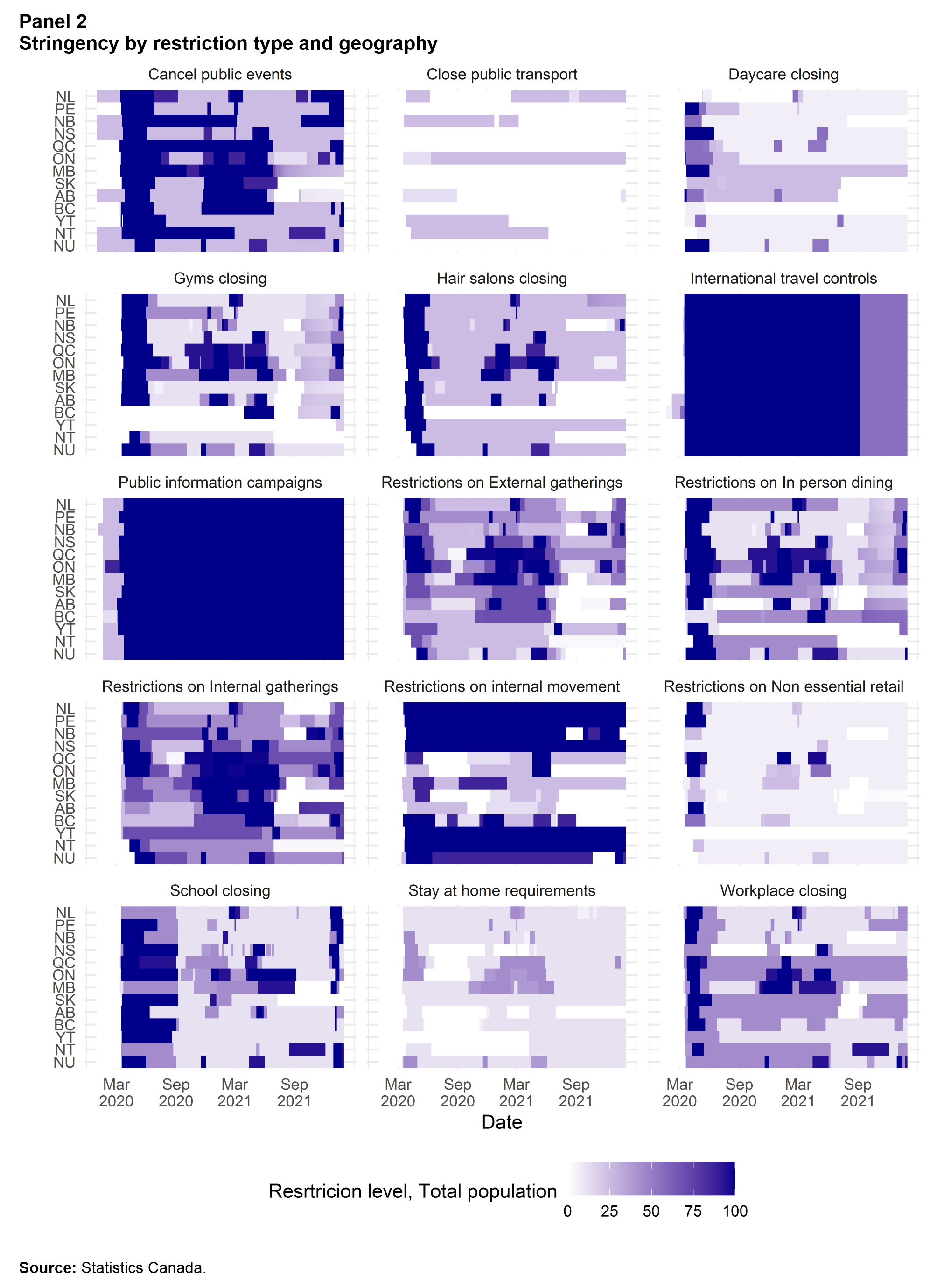
Description for panel 2
Panel 2 shows heat maps for each of the restriction types over time. There are 15 heat maps, one for each of the restriction categories. The heat maps are dark blue when a particular restriction is stringent and white when a restriction is relaxed. The heat maps have provinces and territories on the y-axis. The x-axis of the graphs are days starting with January 01, 2020 and ending with January 31, 2022.
The heat maps show that restrictions on international travel and public information campaigns are common across provinces and territories while changes in business and school restrictions tend to be tighter in Quebec and Ontario than in other provinces, and that these restrictions tend to be in place longer in these jurisdictions.
The data is available in csv format
3.2 Monthly restrictions index versus Labour Force Survey employment, retail sales and active firms
This section provides numerical estimates of the effect of COVID-19 restrictions on Labour Force Survey employment, retail sales and the number of active firms. For all three variables, rising restriction levels lead to declining activity levels, while relaxing restriction levels allows activity levels to rebound. However, the effect is not constant over time and varies across the different waves of the pandemic.
COVID-19 restrictions were introduced to slow the spread of the virus through the population, and the principal means by which restrictions accomplished this was by keeping people apart. Over the course of the pandemic, restrictions were refined, and households and businesses adjusted to their new circumstances. Therefore, the adjustment period at the start of the pandemic had characteristics that were notably different from those in subsequent waves.
The first wave was characterized by a high degree of uncertainty and unpreparedness for the physical distancing measures that were needed to slow the spread of COVID-19. It was also characterized by high degrees of enforcement and cooperation, with the vast majority of Canadians following public health guidelines. As a consequence, the first wave of the pandemic is marked by a strong economic response to rising restriction levels when compared with later waves of COVID-19.
The months that span the second and third waves coincided with adjustments to the restrictions that allowed many businesses to conduct limited operations instead of closing completely, as was generally the case during the first wave. The adjustments took many different forms, depending on the industry and the business. They included moving to remote work arrangements, introducing capacity limits in facilities, and introducing physical distancing measures and increased sanitation. Coincidentally, public health authorities refined their restriction measures, pursuing more measured, or mixed, responses to changes in case counts. This is the approach currently in place.

Data table for Chart 1
| Restriction index | Employment | |
|---|---|---|
| 2020 | ||
| January | 1.5 | 7,491 |
| February | 7.2 | 7,495 |
| March | 35.0 | 7,096 |
| April | 82.5 | 6,405 |
| May | 73.9 | 6,372 |
| June | 64.1 | 6,737 |
| July | 54.7 | 6,884 |
| August | 42.5 | 6,999 |
| September | 33.3 | 7,172 |
| October | 43.4 | 7,199 |
| November | 51.1 | 7,225 |
| December | 68.2 | 7,233 |
| 2021 | ||
| January | 74.8 | 7,085 |
| February | 70.6 | 7,198 |
| March | 61.9 | 7,368 |
| April | 74.7 | 7,215 |
| May | 82.1 | 7,206 |
| June | 62.3 | 7,311 |
| July | 40.9 | 7,368 |
| August | 33.9 | 7,416 |
| September | 27.7 | 7,500 |
| October | 28.6 | 7,529 |
| November | 36.7 | 7,587 |
| December | 37.7 | 7,639 |
| 2022 | ||
| January | 51.0 | 7,494 |
| Source: Statistics Canada. | ||
Data on restrictions and employment for Ontario illustrate how the first wave differs from later waves (Chart 1). The level of restrictions rose very quickly in March and April 2020, when the pandemic began, and reached its highest level on record in April 2020. As restrictions were implemented during the first wave of COVID-19, employment fell sharply according to the Labour Force Survey, reaching its lowest point in May 2020. After April and May 2020, employment began to recover as restrictions began to ease. Gains were rapid at first, and then became more gradual. Beginning in the fall of 2020, restrictions once again began to tighten. However, rather than declining, employment growth in the province slowed. This period of slower growth continued until December 2020, when restrictions tightened to levels similar to those from the height of the first wave. Beginning in December, tighter restrictions led to declining employment, and a negative correlation between restrictions and employment emerged as restrictions, which remained elevated, were eased and tightened over the following months.
This same relationship, where the response is initially stronger and then wanes, emerges in varying degrees for all provinces and territories. Correlations between the severity of restrictions and retail sales, or between employment and the number of active firms are always stronger when the first wave is included in the calculation (Table 2). In many cases, including the first wave more than doubles the correlation between the restrictions index and the economic data, and serves to highlight both the strength of the relationship during the first wave and the more mixed responses over the subsequent waves.
| Retail sales | Employment | Active firms | ||||
|---|---|---|---|---|---|---|
| First wave | After first wave | First wave | After first wave | First wave | After first wave | |
| (Jan. 2020 to Jun. 2020) | (Jul. 2020 to May 2021) | (Jan. 2020 to Jun. 2020) | (Jul. 2020 to May 2021) | (Jan 2020. to Jun. 2020) | (Jul. 2020 to May. 2021) | |
| percent change | ||||||
| British Columbia | -0.99 | -0.49 | -0.99 | -0.63 | -0.91 | -0.35 |
| Alberta | -0.97 | -0.35 | -0.99 | -0.75 | -0.85 | -0.06 |
| Saskatchewan | -0.95 | -0.04 | -0.98 | -0.84 | -0.96 | 0.18 |
| Manitoba | -0.91 | -0.35 | -1.00 | -0.80 | -0.98 | -0.51 |
| Ontario | -0.98 | -0.50 | -0.91 | -0.69 | -0.87 | -0.47 |
| Quebec | -0.92 | -0.23 | -0.99 | -0.60 | -0.99 | -0.25 |
| New Brunswick | -0.95 | 0.47 | -1.00 | 0.21 | -1.00 | 0.25 |
| Prince Edward Island | -0.96 | -0.47 | -0.99 | -0.12 | -0.97 | 0.05 |
| Nova Scotia | -0.96 | -0.86 | -1.00 | -0.86 | -0.86 | -0.60 |
| Newfoundland and Labrador | -0.97 | -0.32 | -0.98 | -0.65 | -0.89 | -0.23 |
| Nunavut | 1.00 | 0.01 | -0.95 | -0.45 | 0.48 | -0.44 |
| Northwest Territories | -0.70 | -0.72 | -0.40 | 0.27 | -0.59 | -0.33 |
| Yukon | -0.88 | -0.23 | 0.45 | 0.30 | -0.63 | -0.08 |
| Average | -0.78 | -0.31 | -0.83 | -0.43 | -0.77 | -0.22 |
| Source: Statistics Canada. | ||||||
Therefore, the pattern that emerges shows how the effects of restrictions during the first wave are very strong compared with later periods. After the first wave, lower but rising levels of restrictions appear to slow growth. This pattern also shows how restrictions appear to have a much stronger effect above a given threshold. In this pattern, determining the effect of rising or falling restrictions on economic activity is not straightforward.
3.2.1 Threshold effects
During the second and third waves of the pandemic, it appears that rising restrictions lead to slower growth up to a point, and that once that point is crossed, rising restrictions correspond with declines in economic activity.
Panel 3 shows the correlation between the growth of the restrictions index and growth in employment, retail sales and the number of active firms for different threshold values. Beginning with an index value of 20, the correlation is calculated using the subset of the data for which the restriction level is above the potential threshold value. The correlation is calculated for all index values between 20 and 60. When the correlations are calculated including the first wave, a clear break in the correlations occurs at the restrictions index value of 41. When data from the first wave are excluded, it becomes less clear where the threshold lies. The correlations strengthen and become increasingly negative in steps for employment and retail sales between index values of around 32 and 60, with the value of 41 as the approximate midpoint of the first long decline. For active firms, there is a discontinuity at around 41. At a value of 41, restrictions tend to go from being an inconvenience (e.g., wear a mask and gather only in small groups) to being a burden (e.g., in-person schooling is cancelled, nonessential retail and personal services are closed, and stay-at-home orders are issued). The value of 41, therefore, represents a point at which restrictions tend to become more binding for personal and business activities, and thus represents a level above which increases in restrictions can lead to more noticeable changes in activity. For the pooled data, the correlations suggest that when index values are below 41, increasing restrictions is associated with slightly slower growth. Furthermore, when index values are above a value of 41, increasing restrictions is associated with larger declines in growth for employment, retail sales or the number of active firms. If the increase in restrictions above the threshold is large enough, there can be negative growth associated with the change.
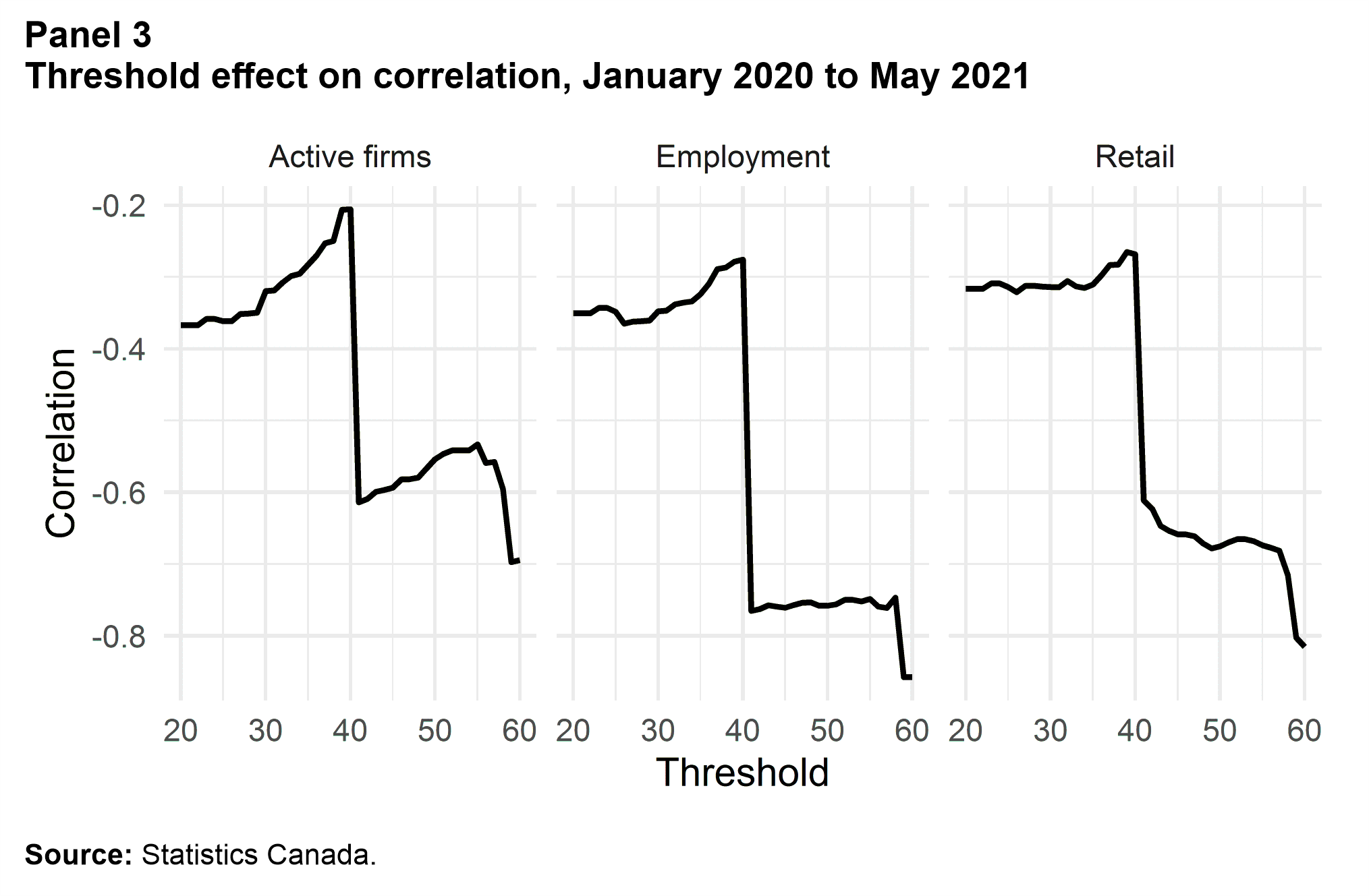
Description for panel 3
Panel 3 has three line graphs, one each for of three variables: retail sales, employment, and the number of active firms. The graphs have the correlation between growth rates for the variables and the growth rate of the total population restrictions index. The y-axis represents the correlation, and spans from -0.2 to -0.9. The x-axis has threshold values based on the level of the index ranging from 20 to 60. The charts includes data on the first, second and third waves of COVID-19.
The line graphs show a distinct change in the correlation between the growth in the variables and the growth of restrictions around a value of 41. This disjoint movement in the line represents a level of the index at which the correlation between variable growth and changes in restrictions becomes stronger.
The data is available in csv format

Description for panel 4
Panel 4 has the same structure as Panel 3. It has three line graphs, one each for of three variables: retail sales, employment, and the number of active firms. The graphs show the correlation between growth rates for the variables and the growth rate of the total population restrictions index. The y-axis represents the correlation, and spans from -0.2 to -0.9. The x-axis has threshold values based on the level of the index ranging from 20 to 60. The charts only include data after the first wave of COVID-19.
The line graphs in Panel 4 show a gradual change in the correlation between the growth in the retail sales and employment with a mid-point around a value of 41. The correlation between changes in the active firm population and changes in restrictions has some variability, but is essentially flat for most of the possible threshold values. The chart illustrates that threshold is less prevalent when the first wave of COVID-19 is excluded.
The data is available in csv format
3.2.2 Regression results
Although comparing the indexes with economic variables and exploring their correlations clearly shows that the restrictions are associated with changes in economic activity, this type of analysis does not allow for an understanding of how large an effect, in percentage points, changing restriction levels could have on economic activity. For a numerical effect, a statistical model must be used.
However, a statistical model requires enough relevant data to produce a reliable estimate. Limited data are available on the effects of the restrictions, which affects whether statistical models can provide precise estimates. Additionally, the stronger response to the first wave of COVID-19 compared with later responses suggests that the first wave will act as an outlier that overstates the effect of rising restrictions for the current economic situation. To understand the current economic response to changing restriction levels, the first wave of COVID-19 is therefore removed from the sample.Note In this present study, the second and third waves are dated from June 2020 to May 2021. This provides 12 data points for each province.
Because of the limited number of observations, data from the provinces are combined to estimate the effect of changing restriction levels on employment, retail sales and the number of active firms.Note This produces an average effect rather than a province-specific effect. However, given the small amount of available data, this method makes it possible to estimate more robust responses. Combining the data in this way produces a longitudinal dataset with repeated measures of the variables for each of the provinces.
The size of the response is then estimated using a linear equation with a threshold effect:
where is employment, retail sales or active firms; is provinces; is time; and is 1 if is greater than or equal to 41, and is 0 if otherwise. Using log differences in the estimating equation makes it easier to interpret the parameters, since the coefficient () represents the percentage point change in a dependent variable for a 1% change in the restrictions index. Similarly, estimates the change in a dependent variable for a 1% change in the restrictions index when the index is above 41.0.
Three estimators are used to gauge the size of the effect on economic variables from changing restriction levels. The first is the ordinary least squares (OLS) estimator, the second is the fixed effects (FE) estimator, and the third is the random effects (RE) estimator. The OLS estimator pools the data to provide an average response across provinces and territories and imposes the restriction that . Since the model is defined as log differences, this is equivalent to assuming that the underlying growth not related to COVID-19 in all provinces is the same during this period.
The FE and RE estimators are longitudinal estimators that allow for province-specific average growth rates. The difference between the FE and RE estimates comes from the interpretation of the differing average growth rates. The FE estimator assumes that the average growth rates are deterministic, while the RE estimator assumes that the province specific average growth rates are random variables. The FE and RE models allow for more sophisticated use of the available data, but the limited number of time periods (only data from June 2020 to August 2021 are available) affects the capacity of the models to provide robust province-specific estimates.
The results for employment, retail trade and the number of active firms are reported in tables 3, 4 and 5, respectively. An F-test and the Breusch-Pagan Lagrange Multiplier (LM) tests are used to test whether it can be reasonably assumed that the average growth rate is the same. The Hausman F-test is reported to test whether or not the province-specific growth rates are better treated as deterministic or random. During reporting, if the hypothesis that the average growth rates are the same is rejected, then the tests are examined for the preferred panel model.
For retail sales, the tests suggest that the RE model is most appropriate. The F-test and LM test both suggest that average growth rates differ across the provinces, and the Hausman test suggests that the growth rates should be treated as random. The result is a parameter estimate of -0.04 for changes in the restrictions index that rises to -0.1 once the index threshold of 41 has been passed. For employment, the tests suggest that the OLS model is most appropriate. The F-test and LM test both support the hypothesis that average growth rates during the period are not statistically different. The result is a parameter estimate of -0.02 that rises to ‑0.06 above the index threshold value of 41. For active firms, the tests also suggest that the OLS model is most appropriate. The F-test and LM test fail to reject the hypothesis that the average growth rates are the same, leading to a parameter estimate of -0.01 that is largely unchanged above the index threshold value of 41.
The results show a weaker effect when the index is below the threshold value of 41, but rises for retail sales and employment once restrictions surpass the index value of 41. Intuitively, the threshold value represents the level at which restrictions become binding for economic activity. This can occur either because a wide range of restrictions is in place or, more commonly, because restriction levels rise to a point in which they become binding for businesses. Once restriction levels rise beyond the threshold level, growth of 10 percentage points in the restriction indexes correspond to a 1.0 percentage point decline in retail sales growth and a 0.6 percentage point decline in employment growth.
Caution is warranted when interpreting the regression results. There are limited data, and the error terms exhibit heteroscedasticity. The model itself is simple and has likely omitted variable bias. As a result, the inference in this study is not strong. While the coefficient signs and magnitudes are appropriate, confidence intervals for coefficients usually contain 0. Taken together, the results are informative and suggest correlations between changes in restrictions and changes in economic variable growth. However, more data and more complex models are needed before greater confidence can be attached to estimation strategies and parameter values. At this time, the reported results provide a preliminary indication of the size and direction of the effect restrictions have on economic variables, but this may change as more data and better models become available.
| Pooled OLS | Fixed effects | Random effects | |
|---|---|---|---|
| Regression coefficent | -0.020 | -0.050 | -0.040 |
| Standard error | -0.039 | -0.045 | -0.039 |
| 95% confidence interval | |||
| Lower bound | -0.100 | -0.140 | -0.120 |
| Upper bound | 0.053 | 0.034 | 0.037 |
| Regression coefficent | -0.100 | -0.040 | -0.060 |
| Standard error | -0.050 | -0.054 | -0.048 |
| 95% confidence interval | |||
| Lower bound | -0.200 | -0.140 | -0.150 |
| Upper bound | 0.001 | 0.070 | 0.035 |
| -0.120 | -0.090 | -0.100 | |
| R-squared | 0.160 | 0.110 | 0.130 |
|
Note: OLS refers to ordinary least squares. Source: Statistics Canada, authors' calculations. |
|||
| Hypothesis | Test | Statistic |
|---|---|---|
| p-value | ||
| Ho:
for all i Ha: for all i |
F-test | 0.01 |
| Ho: Ha: |
Breusch-Pagan Lagrange Multiplier test | 0.04 |
| Ho:
are random Ha: are deterministic |
Hausman F-test | 0.60 |
| Ho: Ha: |
Similarity in average growth rates | |
| Pooled OLS | 0.86 | |
| Fixed effects | 0.86 | |
| Random effects | 0.86 | |
|
Note: OLS refers to ordinary least squares. Ho is null hypothesis and Ha is alternative hypothesis. Source: Statistics Canada, authors' calculations. |
||
| Pooled OLS | Fixed effects | Ramdom effects | |
|---|---|---|---|
| 10% increase in the restrictions index (threshold > 41) |
|||
| Regression coefficient | -1.2 | -0.9 | -1.0 |
| 95% confidence interval | |||
| Lower bound | -3.0 | -2.8 | -2.7 |
| Upper bound | 0.5 | 1.0 | 0.7 |
| 20% increase in the restrictions index (threshold > 41) |
|||
| Regression coefficient | -2.4 | -1.8 | -2.0 |
| 95% confidence interval | |||
| Lower bound | -5.9 | -5.6 | -5.4 |
| Upper bound | 1.1 | 2.1 | 1.4 |
|
Note: OLS refers to ordinary least squares. Source: Statistics Canada, authors' calculations. |
|||
| Pooled OLS | Fixed effects | Random effects | |
|---|---|---|---|
| Regression coefficent | -0.02Note * | -0.01 | -0.02 |
| Standard error | -0.01 | -0.01 | -0.01 |
| 95% confidence interval | |||
| Lower bound | -0.05 | -0.04 | -0.04 |
| Upper bound | -0.001 | -0.010 | 0.003 |
| Regression coefficent | -0.04Note * | -0.04Note * | -0.04Note ** |
| Standard error | -0.01 | -0.02 | -0.01 |
| 95% confidence interval | |||
| Lower bound | -0.060 | -0.073 | -0.070 |
| Upper bound | -0.009 | -0.007 | -0.009 |
| -0.06 | -0.05 | -0.06 | |
| R-squared | 0.38 | 0.30 | 0.34 |
Source: Statistics Canada, authors' calculations. |
|||
| Hypothesis | Test | Statistic |
|---|---|---|
| p-value | ||
| Ho:
for all i Ha: for all i |
F-test | 0.2 |
| Ho: Ha: |
Breusch-Pagan Lagrange Multiplier test | 0.2 |
| Ho:
are random Ha: are deterministic |
Hausman F-test | 0.6 |
| Ho: Ha: |
Similarity in average growth rates | |
| Pooled OLS | 0.06 | |
| Fixed effects | 0.06 | |
| Random effects | 0.06 | |
|
Note: OLS refers to ordinary least squares. Ho is null hypothesis and Ha is alternative hypothesis. Source: Statistics Canada, authors' calculations. |
||
| Pooled OLS | Fixed effects | Ramdom effects | |
|---|---|---|---|
| 10% increase in the restrictions index (threshold > 41) |
|||
| Regression coefficient | -0.6 | -0.5 | -0.6 |
| 95% confidence interval | |||
| Lower bound | -1.1 | -1.1 | -1.1 |
| Upper bound | -0.1 | 0.0 | -0.1 |
| 20% increase in the restrictions index (threshold > 41) |
|||
| Regression coefficient | -1.1 | -1.0 | -1.0 |
| 95% confidence interval | |||
| Lower bound | -2.0 | -2.0 | -1.9 |
| Upper bound | -0.20 | 0.09 | -0.10 |
|
Note: OLS refers to ordinary least squares. Source: Statistics Canada, authors' calculations. |
|||
| Pooled OLS | Fixed effects | Random effects | |
|---|---|---|---|
| Regression coefficent | -0.01Note * | -0.02Note * | -0.003 |
| Standard error | -0.007 | -0.007 | -0.005 |
| 95% confidence interval | |||
| Lower bound | -0.03 | -0.03 | -0.01 |
| Upper bound | -0.002 | -0.003 | 0.008 |
| Regression coefficent | 0.005 | 0.007 | -0.005 |
| Standard error | -0.008 | -0.009 | -0.006 |
| 95% confidence interval | |||
| Lower bound | -0.01 | -0.01 | -0.02 |
| Upper bound | 0.020 | 0.020 | 0.009 |
| -0.009 | -0.009 | -0.006 | |
| R-squared | 0.081 | 0.096 | 0.030 |
Source: Statistics Canada, authors' calculations. |
|||
| Hypothesis | Test | Statistic |
|---|---|---|
| p-value | ||
| Ho:
for all i Ha: for all i |
F-test | 0.8 |
| Ho: Ha: |
Breusch-Pagan Lagrange Multiplier test | 0.4 |
| Ho:
are random Ha: are deterministic |
Hausman F-test | 0.002 |
| Ho: Ha: |
Similarity in average growth rates | |
| Pooled OLS | 0.005 | |
| Fixed effects | 0.005 | |
| Random effects | 0.005 | |
|
Note: OLS refers to ordinary least squares. Ho is null hypothesis and Ha is alternative hypothesis. Source: Statistics Canada, authors' calculations. |
||
| Pooled OLS | Fixed effects | Ramdom effects | |
|---|---|---|---|
| 10% increase in the restrictions index (threshold > 41) |
|||
| Regression coefficient | -0.1 | -0.1 | -0.1 |
| 95% confidence interval | |||
| Lower bound | -0.4 | -0.4 | -0.3 |
| Upper bound | 0.2 | 0.2 | 0.2 |
| 20% increase in the restrictions index (threshold > 41) |
|||
| Regression coefficient | -0.2 | -0.2 | -0.1 |
| 95% confidence interval | |||
| Lower bound | -0.8 | -0.8 | -0.6 |
| Upper bound | 0.4 | 0.4 | 0.3 |
|
Note: OLS refers to ordinary least squares. Source: Statistics Canada, authors' calculations. |
|||
4 Conclusion
The restrictions index presented in this study builds on the Oxford Stringency Index, but makes four important modifications. First, the input variables are adjusted to better reflect provincial and territorial experiences. In some cases, such as gathering sizes, a distinction is made between internal and external restrictions. Additionally, bin sizes are changed to better reflect how provincial and territorial health authorities implemented restrictions. New variables, such as closures for nonessential retail establishments, are added as well. Second, new variables are implemented to better reflect Canadian restrictions. Third, an adjustment is made to produce differences between the vaccinated and unvaccinated populations. Finally, the input values for the index are squared to allow for the larger marginal effects of moving to progressively tighter restrictions.
The results produce an index at a daily frequency that tracks the provincial and territorial restrictions for COVID-19. The index values clearly show differences in the severity of restrictions across the provinces and different industries during different waves of the pandemic. The indexes highlight more severe restriction measures in central Canada and comparatively less severe measures in British Columbia and Alberta. They also show that more common restrictions have tended to be implemented on personal activity (e.g., gathering sizes and movement) and on some forms of business activity (e.g., nonessential retail and personal services). Furthermore, a differentiation between restrictions on the vaccinated and unvaccinated populations emerges once vaccines become widely available, with the largest differences arising in Manitoba and Ontario.
However, care should be exercised in drawing strong conclusions about whether or not one province or territory has more stringent restrictions than another when using the index in isolation. The index categories are created to compare actions over time and across geographies. This creates a measurement challenge as different forms of restrictions will sometimes need to be grouped together to promote comparability (for example with restrictions on movement that include curfews and community closures) and when restrictions are enacted differently as the pandemic evolves (for example with the introduction and updating of color coded systems). Moreover, there is no account for adherence or enforcement. So, while the index is instructive, in cases where there is uncertainty when comparisons are made, additional information should be used to make conclusions.
The daily index can be averaged to a monthly frequency to understand how restrictions and monthly economic variables are related. Here, the impact of restrictions on employment, retail sales and the number of active firms is examined. The results show that the response of economic variables to restrictions during the first wave of COVID-19 was stronger than in the later waves. This is likely because households and businesses adapted to physical distancing, capacity limits and increased sanitation, as well as governments refined their restrictions.
Using pooled data from the second and third waves of COVID-19, statistical models suggest that when the level of restrictions is low, increasing restrictions acts to slow growth. After restrictions reach a threshold value of 41, however, they begin to have a larger impact, and are associated with declines in economic activity. At a value of 41, restrictions tend to go from being an inconvenience (e.g., wear a mask and gather only in smaller groups) to being a burden (e.g., in-person schooling is cancelled, nonessential retail and personal services are closed, and stay-at-home orders are issued). The value of 41, therefore, represents a point at which restrictions tend to become more binding for personal and business activities, and thus represents a level above which increases in restrictions can lead to more noticeable changes in activity. Numerically, the models suggest that below the threshold value, growth of 10 percentage points in the restrictions index is associated with retail sales growth slowing by about 0.4 percentage points, with employment growth slowing by 0.2 percentage points, and with the growth rate in the number of active firms slowing by 0.1 percentage points. Once restriction levels surpass the threshold value, growth of 10 percentage points in the restrictions index is associated with retail sales growth slowing by 1.0 percentage points, with employment growth slowing by 0.6 percentage points, but the response of the active firm growth rate is little changed at a reduction of 0.1 percentage points. The reason why active firms are less affected by the threshold after the first wave is not clear, but it may relate to government support programs keeping business open, or to adaptation to work spaces that permit operation during the pandemic or to effects from the first wave that have persisted over time.
Finally, a limitation of the analysis is that a large part of the variation in the data needed to identify the relationship between restrictions and economic variables comes from the number of waves of the pandemic. Additional waves of the pandemic would provide more information, but the strength of the relation between restrictions and economic variables is likely to change as businesses and consumers continue to adapt.
5 Works cited
[1] Hale, T., Anania, J., Angrist, N., Boby, T., Cameron-Blake, E., Di Folco, M., Ellen, L., Goldszmidt, R., Hallas, L., Kira, B., Luciano, M., Majumdar, S., Nagesh, R., Petherick, A., Phillips, T., Tatlow, H., Webster, S., Wood, A., & Zhang, Y. (2021, June 11). Variation in government responses to COVID-19. Blavatnik School of Government Working Paper, Version 12.https://www.bsg.ox.ac.uk/sites/default/files/2021-06/BSG-WP-2020-032-v12_0.pdf
[2] Cheung C., Lyons, J., Madsen, B., Miller, S., & Sheikh, S. (2020). The Bank of Canada COVID‑19 stringency index: measuring policy response across provinces.Staff Analytical Notes 2021-1. Bank of Canada.
[3] Cameron-Blake, E., Breton, C., Sim, P., Tatlow, H., Hale, T., Wood, A., Smith, J., Sawatsky, J., Parsons, Z., & Tyson, K. (2021). Variation in the Canadian provincial and territorial responses to COVID-19. (Working paper, No. BSG-WP-2021/039). Centre of Excellence on the Canadian Federation.
- Date modified: