
Analytical Studies: Methods and References
Developing Meaningful Categories for Distinguishing Levels of Remoteness in Canada
by Rajendra Subedi, Shirin Roshanafshar and T. Lawson Greenberg
Centre for Population Health Data (CPHD) No. 026
Skip to text
Text begins
Acknowledgements
We would like to thank Erin Pichora from the Canadian Institute for Health Information, and Alessandro Alasia and François Sergerie from Statistics Canada for their valuable comments and suggestions as official reviewers of this paper.
Abstract
The concepts of urban and rural are widely debated and vary depending on a country’s geopolitical and sociodemographic composition. In Canada, population centres and statistical area classifications are widely used to distinguish urban and rural communities. However, neither of these classifications precisely classify Canadian communities into urban, rural and remote areas. A group of researchers at Statistics Canada developed an alternative tool called the “remoteness index” to measure the relative remoteness of Canadian communities. This study builds on the remoteness index, which is a continuous index, by examining how it can be classified into five discrete categories of remoteness geographies. When properly categorized, the remoteness index can be a useful tool to distinguish urban, rural and remote communities in Canada, while protecting the privacy and confidentiality of citizens. This study considers five methodological approaches and recommends three methods.
Keywords: remoteness, urban, rural, classification, natural break, clusters
1 Introduction
The concepts of urban and rural have been widely debated throughout the world. The definitions of urban and rural vary depending on a country’s geopolitical situation and sociodemographic composition. Some researchers have defined “rural” as communities defined by geography that have unique demographic structures and settlement patterns, isolated populations, long commuting distances, limited supplies of goods and services, and mostly agriculture-based and natural-resource-based economies (Hart, Lishner and Larson 2005; Johnson and Johnson 2015; du Plessis et al. 2002). However, there are no universally accepted definitions of urban and rural, and there is no universally accepted urban, rural and remote classification.
In general, countries have defined rural and remote areas in terms of geographic accessibility and population density. For example, in the United States, counties and county-equivalent entities with populations of less than 10,000 are classified as non-core counties, and are generally considered rural areas (NCHS 2014). In the United Kingdom, the 2011 Rural Urban Classification defined any output area with a population of 10,000 or more as urban, and the remaining output areas were defined as rural (Bibby and Brindley 2013). However, the criteria applied in the United States and the United Kingdom are not applicable in the Canadian context since the population density in Canada is comparatively low.
In Australia, there are three accessibility and remoteness measures: the Rural Remote and Metropolitan Area geographic classification (DPIE and DHSH 1994), the Accessibility/Remoteness Index of Australia (Department of Health and Aged Care 2001), and the Australian Standard Geographical Classification (AIHW 2004). All three classifications divide Australian geography into urban, rural and remote areas based on accessibility to a range of services.
In Europe, however, much of the territory does not fit in an urban–rural dichotomy, and instead falls in between urban–rural typology, mainly because of densely populated rural areas (Wandl et al. 2014). National statistical agencies in European countries use different definitions of urban and rural. Therefore, urban and rural areas vary widely between countries (Peen et al. 2010).
In the Canadian context, the most common urban–rural classification is the concept of population centres (POPCTRs)Note (previously “urban areas”). POPCTRs have been used by Statistics Canada since 2011, and are most often used for demographic studies in Canada. All communities outside POPCTRs are considered rural. Although POPCTRs are classified into three groups—small (with populations of 1,000 to 29,999), medium (with populations of 30,000 to 99,999) and large (with populations of 100,000 or more)—they do not account for differences between small urban centres and metropolitan areas with populations of more than 1 million.
POPCTRs classify all communities with a population of less than 1,000—or a density of less than 400 people per square kilometre—as rural, despite the fact that some of these areas benefit from their close proximity to large urban centres. Therefore, the concept of POPCTRs takes into account population size and density, but ignores proximity to large urban centres that provide goods and services to small towns. Furthermore, one of the major disadvantages of using POPCTRs in urban–rural classification is that they are created based on dissemination blocks, which cannot accurately be assigned to postal codes for about 25% of the population (primarily those living in urban fringe and rural areas) (Statistics Canada 2017).
Statistics Canada developed the remoteness index (RI) in 2017 to complement existing geographic classification methods (see Alasia et al. 2017). Although this paper aims to develop discrete RI categories, other geographic classification methods are also discussed to provide information on the background and limitations of the existing methods. The RI provides relative remoteness values for almost all Canadian census subdivisions (CSDs). This cannot be done using POPCTRs because POPCTR boundaries do not exactly correspond to CSD boundaries. For example, five POPCTRs straddle provincial boundaries, but all CSDs follow provincial or territorial boundaries (Statistics Canada 2016a).
Another geographic classification method used in Canada is the Statistical Area Classification (SAC), which groups CSDs according to whether they are part of a census metropolitan area (CMA), a census agglomeration (CA), a metropolitan influenced zone (MIZ) or Territories (Statistics Canada 2016b). A MIZ is further divided into four categories according to degree of influence (strong, moderate, weak and no influence), based on the percentage of the population that commutes to work in one or more of the CMAs or CAs. The underlying assumption of the SAC is that more people tend to commute to work if they live near a CMA or CA. The SAC is most often used to report on health indicators or other data where place-of-residence information is limited to postal code. However, the SAC does not precisely measure the access to goods and services available within or in proximity to a community. Furthermore, the SAC groups together all CSDs within the territories, despite the fact that some areas are more accessible than others.
The concept of remoteness is especially relevant in the study of socioeconomic characteristics and population health status because the geographic information in health data is often limited to residential postal code. Studies have shown that rural and remote populations experience poorer health, higher mortality, lower life expectancy and higher unmet healthcare needs (Eckert, Taylor and Wilkinson 2004; Mitura and Bollman 2003). For example, an analysis by the Canadian Institute for Health Information (CIHI) suggests that there are disproportionately higher rates of hospitalizations and mortality caused by asthma, chronic obstructive pulmonary disease, diabetes, high blood pressure and heart disease among people living in rural areas compared with those living in urban areas, even after accounting for higher disease prevalence rates (CIHI 2012). An earlier CIHI analysis examined the health status of Canadians by degree of rurality using MIZs (DesMeules and Pong 2006). However, the study used moderate and weak MIZs, and the territories, as remote areas.
The newly developed RI could be a more reliable alternative to the traditional POPCTR and SAC geographic classification concepts for Canada because it assigns a relative remoteness value to each CSD, based on proximity to agglomerations.
In 2018, the RI was updated to reflect the 2016 geographies and populations of CSDs. It measured the relative remoteness of each CSD on a normalized scale of 0 to 1, where 0 is the most accessible (urban) area and 1 is the least accessible (remote) area. One of the advantages of the RI is that it can be updated after each Census of Population, which occurs every five years.
Although the RI is a useful concept for understanding the relative remoteness of each CSD, its continuous scale is less useful for disseminating statistical information, unless CSDs are grouped together into a few categories with similar remoteness indexes. A meaningful grouping of RI values would help to disseminate health and socioeconomic indicators, without the risk of compromising the privacy and confidential information of individuals.
The objective of this methodology paper is to explore different approaches for categorizing the continuous RI values of Canadian CSDs into meaningful groups, and to recommend a few classifications that are suitable for future use. These classifications can complement traditional urban–rural classifications. This paper explores five methodological approaches for classifying remoteness into five discrete categories. The methods considered are manual classification, equal interval classification, quantile classification, Jenks natural breaks classification and k-means cluster classification. Each method is used to aggregate CSDs with similar RI values to form meaningful remoteness categories.
2 Data and methods
The dataset used in this classification is the updated RI that reflects 2016 CSD geographies and populations (Alasia et al. 2017). The RI was developed by combining data from official statistical sources like the Census of Population with data from non-official statistical sources such as Google Map API. The RI takes a CSD as geographic units of analysis, and the index value was computed by combining the geographic layers of the CSD and the POPCTR. Each CSD’s RI value was determined based on the CSD’s relative proximity (measured in travel costNote ) to all surrounding POPCTRs within a 200-kilometre radius. The population size of each POPCTR was used as a proxy of service availability. The RI calculation accounts for all POPCTRs that could be potential locations for goods, services and economic activities for the reference CSD. The updated RI included index values for all CSDs in Canada that reported a population in 2016, or that were connected to the main transportation network (5,125 out of 5,162 CSDs).
The following figure shows the distribution of RI values of CSDs in 2016. As shown in Figure 1, many CSDs had RI values of 0.10 to 0.14. All of these CSDs were in Quebec, Ontario, Alberta and British Columbia, around densely populated metropolitan areas. Despite having low to medium population sizes, these CSDs had low RI values because of their proximity to large CMAs.

Description for Figure 1
Figure 1 represents the distribution of Canadian census subdivisions (CSDs) by remoteness index (RI), with RI values on the X-axis and percentages on the Y-axis. RI values are normalized in a range of 0 to 1, where 0 represents more accessible areas and 1 represents very remote areas. The RI value given to each CSD is plotted in the graph to determine whether the CSD is distributed normally. The blue columns represent the percentage of CSDs with specific ranges of RI values. The bell-shaped red trend line represents the distribution of the RI values that are close to a normal distribution, with a slight right skewness.
Preliminary work explored the optimal number of categories for a discrete classification. Continuous RI values were classified into different categories using various methods. These methods categorized the RI value into 3 to 10 different categories. When the RI values were classified into fewer than five categories, it was difficult to distinguish urban, rural and remote areas precisely because Canada’s geography extends from core urban centres to very remote areas with no population. In addition, having fewer than five categories made the classification approach similar to the traditional SAC and POPCTRs approaches, in terms of the number of categories.
Conversely, when more than five categories were formed, the CSDs and populations were distributed disproportionately because some categories were formed with only a few CSDs and small populations. A cluster with a small population and a few CSDs is not suitable because it does not allow for comparisons among CSDs from different remoteness classes. For instance, when the RI values were divided into 10 categories using a k-means cluster analysis, some of the categories were formed with a few CSDs with a small population.
Furthermore, forming more than five categories increased the likelihood that private and confidential information would be disclosed, especially when disseminating data from surveys with small sample sizes, or when reporting on rare conditions. Therefore, it was decided that the main analyses would focus only on classifications with five categories: easily accessible area, accessible area, less accessible area, remote area and very remote area. The SAS Enterprise Guide 7.1 was used to classify the data, and ArcMap 10.5.1 was used to show the geographic distribution of CSDs by category in the maps.
3 Results
Remoteness is a relative, not absolute, concept. The main challenge in the classification process is to determine the cut-off points between categories. Because there are no established criteria to classify a continuous variable into discrete categories based on remoteness, the classification approaches proposed in this paper were selected based on an extensive review of literature. Five classification approaches, each with five categories (easily accessible area, accessible area, less accessible area, remote area and very remote area), were examined and compared based on specificity, research objective and suitability for data dissemination.
3.1 Manual classification of remoteness index values based on natural breaks, population count and distribution of census subdivision
Manual classification manually breaks down RI values into five mutually exclusive categories, while also considering the natural breaks observed in the distribution of RI values (Figure 1). Manual classification looks at the distribution of RI values and manually identifies natural breaks in the data, while also considering the number of CSDs and the population distribution in each class. Almost 88% of the CSDs had RI values lower than 0.55 (on a scale from 0 to 1—where 0 represents the most accessible areas and 1 represents the least accessible areas). Therefore, four out of the five categories were formed within the range of 0 to 0.55. The only category that fell beyond the cut-off point of 0.55 was the “very remote area” category. All the CSDs in the “easily accessible area” and “accessible area” categories were connected by a road or ferry network.
| Remoteness | RI score | Population | CSD | Average population/CSD |
|---|---|---|---|---|
| percent | ||||
| Easily accessible area | <0.1500 | 68.14 | 15.10 | 30,974 |
| Accessible area | 0.1500 to 0.2888 | 19.34 | 21.48 | 6,180 |
| Less accessible area | 0.2889 to 0.3898 | 7.90 | 27.51 | 1,972 |
| Remote area | 0.3899 to 0.5532 | 3.84 | 23.98 | 1,098 |
| Very remote area | >0.5532 | 0.78 | 11.92 | 449 |
|
Notes: RI = remoteness index, CSD = census subdivision. Natural breaks are used in such a way that all CSDs with populations greater than 100,000 are classified under either "easily accessible area" or "accessible area," and all CSDs with populations greater than 20,000 are classified under "easily accessible area," "accessible area" or "less accessible area." CSDs with populations greater than 10,000 are not classified under "very remote area." Source: The data for this table come from the data table from the remoteness index of Canadian census subdivisions (Alasia et al. 2017). |
||||
Total population in each category was also considered during RI value classification, despite the fact that about 82% of the Canadian population lives in urban areas (Statistics Canada 2016c). Cut-off points were devised manually so that all CSDs with a population greater than 100,000 fell into either the “easily accessible area” or the “accessible area” categories. This classification was consistent with the SAC method, where POPCTRs with populations of more than 100,000—with a core population of at least 50,000—are considered CMAs. Similarly, all CSDs with a population greater than 20,000 fell into the “easily accessible area,” “accessible area” or “less accessible area” categories. CSDs with a population greater than 10,000 were not placed in the “very remote area” category.
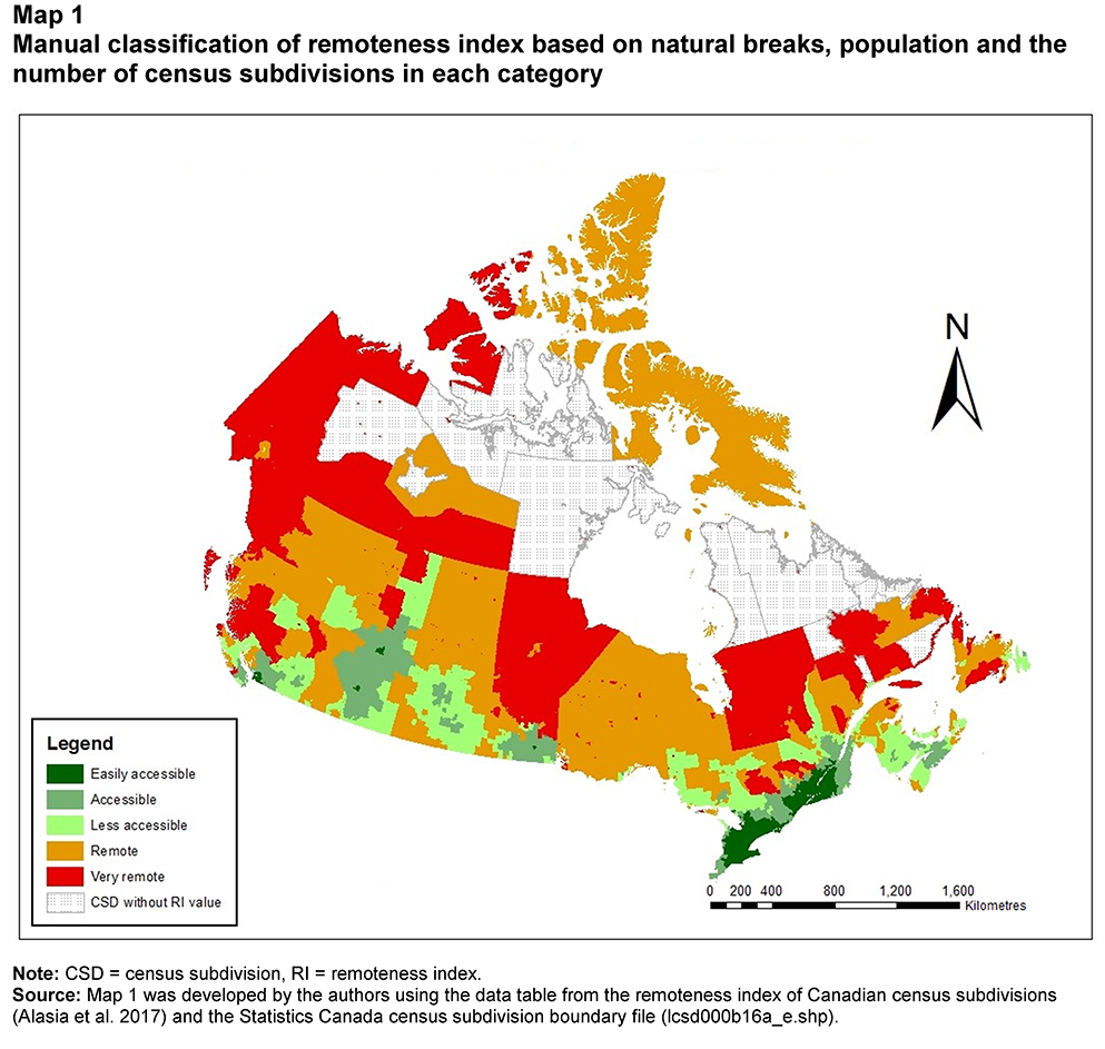
Description for Map 1
Map 1 represents the distribution of Canadian census subdivisions (CSDs) based on the manual classification of the continuous remoteness index (RI) into five discrete categories. The unique value map in a green to red colour ramp was developed using the remoteness class field from the data table. The dark green, green, light green, orange and red colours represent the “easily accessible,” “accessible,” “less accessible,” “remote” and “very remote” areas, respectively. The area with black dots represents CSDs for which the RI values were not available, either because they were not connected to any transportation network or because they did not report any population in the 2016 Census of Population.
One of the major advantages of this classification method is that it separates data into classes based on natural groups in the data distribution, without compromising the distribution of the number of CSDs in each class. For instance, this method of classification assigns at least 12% of CSDs to each category. However, this method is highly subjective. The cut-off points are selected manually and, therefore, need to be updated manually with new census geography and new population information. Another issue with this method is that the urban–rural population distribution is different from what is already known on population distribution in Canada. The “easily accessible area” and “accessible area” categories alone contain more than 87% of the total population, which is more than what is found in all POPCTRs in Canada (Statistics Canada 2016c). However, RI value classification is based on a different approach than the POPCTR approach, and therefore the population distribution may differ by category. The remoteness categories in Table 1 were developed based on the criteria outlined above.
3.2 Equal interval classification based on remoteness index value
Another approach for classifying RI values is the equal interval method, in which five remoteness categories are created by dividing the RI values equally into quintiles. This classification method divides attribute values—in this case, the RI values—into equal value ranges. This method is straightforward and flexible since the number of categories may vary depending on user requirements. This method is also suitable for displaying data that vary linearly, like RI values, and that have no true outliers.
| Remoteness | RI score | Population | CSD | Average population/CSD |
|---|---|---|---|---|
| percent | ||||
| Easily accessible area | <0.20 | 75.36 | 21.01 | 24,618 |
| Accessible area | 0.20 to 0.3999 | 20.56 | 45.66 | 3,091 |
| Less accessible area | 0.40 to 0.5999 | 3.59 | 24.80 | 992 |
| Remote area | 0.60 to 0.7999 | 0.35 | 6.99 | 344 |
| Very remote area | >=0.80 | 0.14 | 1.54 | 642 |
|
Notes: RI = remoteness index, CSD = census subdivision. RI scores by CSD are divided equally into five categories (quintile classification of RI value). Source: The data for this table come from the data table from the remoteness index of Canadian census subdivisions (Alasia et al. 2017). |
||||
However, this method is less suitable than manual classification because the classification is based on the RI value, not the natural breaks in the data. Furthermore, this method does not take into account the population and the number of CSDs in each class. For instance, more than 96% of the population fell into the “easily accessible” or “accessible” categories, which is not consistent with other POPCTR classifications that have been used in Canada. Generally, the average population per CSD decreases as the remoteness increases. However, according to this classification, the average population per CSD in the “remote area” category (344) was lower than the average population per CSD in the “very remote area” (642) category because there were few CSDs in the “very remote area” category.
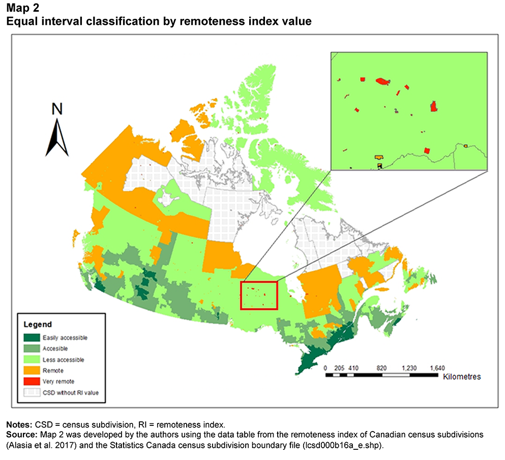
Description for Map 2
Map 2 includes two maps: a map of Canada by census subdivision (CSD), and an inset map of northern Ontario. The map of Canada represents the distribution of CSDs based on the equal interval classification of the continuous remoteness index (RI) into five discrete categories. The unique value map in a green-to-red colour ramp was developed using the remoteness class field from the data table. The dark green, green, light green, orange and red colours represent the “easily accessible,” “accessible,” “less accessible,” “remote” and “very remote” areas, respectively. The area with black dots represents CSDs for which RI values were not available, either because they were not connected to any transportation network, or because they did not report any population in the 2016 Census of Population. The inset map provides a magnified portion of northern Ontario to highlight the few “very remote” areas.
Conversely, over 45% of CSDs fell into the “accessible area” category, while less than 2% fell into the “very remote area” category (some are shown in the magnified portion of Map 2). As a result, some very remote communities in northern Canada were not classified as “very remote” because the RI value did not fall beyond the 0.8 cut-off.
3.3 Quantile classification based on the number of census subdivisions
Another method for classifying RI values is quantile classification based on the total number of CSDs. In this method, an equal number of CSDs are assigned to each of the five categories. A major advantage of this method is that it distributes CSDs equally in each remoteness category, and each category is equally represented on the map. This method is more flexible than others since more than five or fewer than five categories can be formed by simply splitting the number of CSDs equally.
| Remoteness | RI score | Population | CSD | Average population/CSD |
|---|---|---|---|---|
| percent | ||||
| Easily accessible area | <0.1928 | 73.43 | 20.00 | 25,204 |
| Accessible area | 0.1928 to 0.3013 | 15.50 | 20.00 | 5,319 |
| Less accessible area | 0.3014 to 0.3739 | 5.11 | 20.00 | 1,753 |
| Remote area | 0.3740 to 0.4744 | 4.16 | 20.00 | 1,432 |
| Very remote area | >0.4744 | 1.80 | 20.00 | 617 |
|
Notes: RI = remoteness index, CSD = census subdivision. The number of CSDs is divided equally into five categories (quantile classification by CSD). Source: The data for this table come from the data table from the remoteness index of Canadian census subdivisions (Alasia et al. 2017). |
||||
However, the resulting map or data table may be misleading because the CSDs that are put into different classes can have similar RI values, or the CSDs in a same class may have different RI values. Remote CSDs are generally larger than urban CSDs. Therefore, the map is misleading because, with this method, the “very remote area” category is overrepresented. This classification method also compromises the distribution of RI values and population in each category. Since the classification is based on the number of CSDs, it is less useful for population-based studies. Another disadvantage of this method is that many CSDs with a population of more than 10,000 fell into the “very remote area” category since the classification is based on the number of CSDs, not the actual RI value. Therefore, this classification may not accurately represent the actual remote population of Canada.
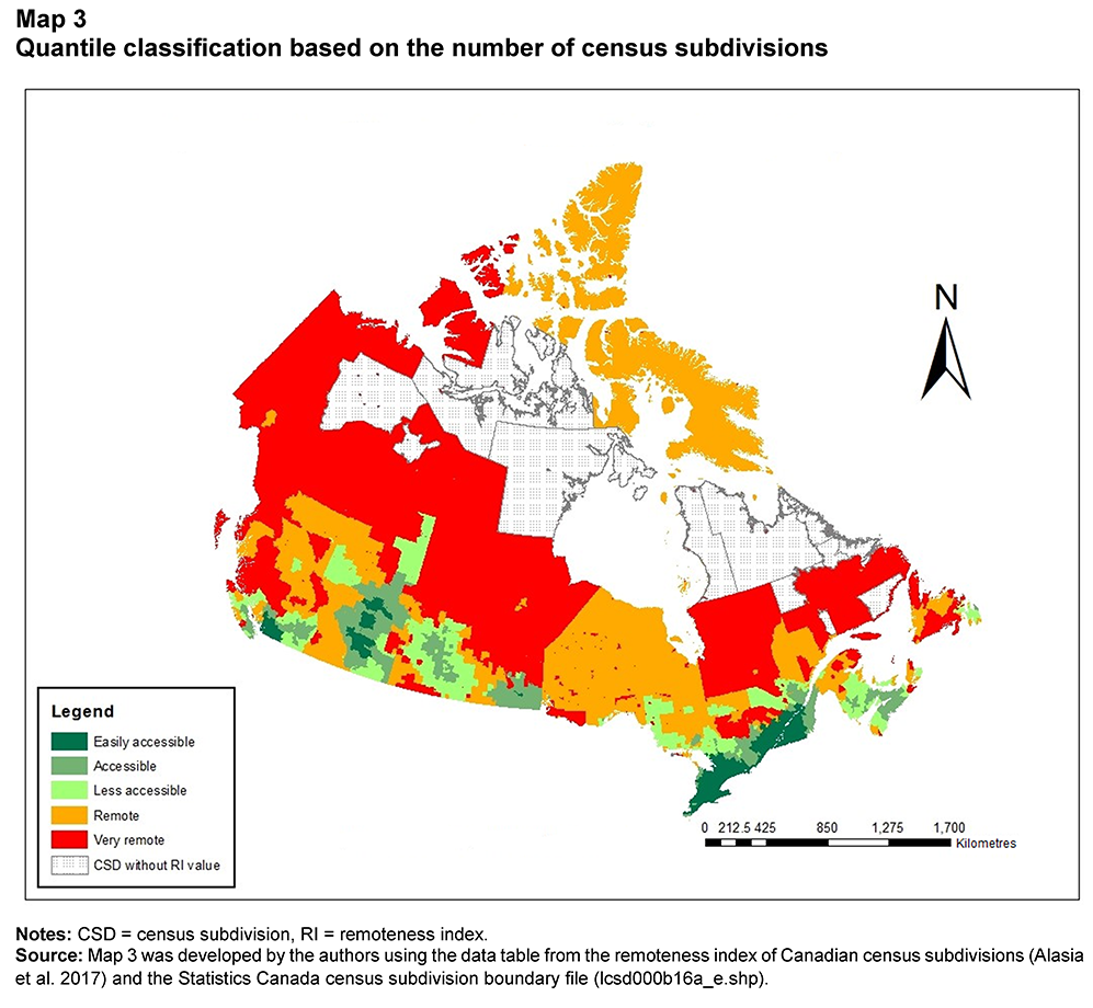
Description for Map 3
Map 3 represents the distribution of Canadian census subdivisions (CSDs) using the quantile classification method. In this method, CSDs are equally classified into five discrete categories. The unique value map in a green-to-red colour ramp was developed using the remoteness class field from the data table. The dark green, green, light green, orange and red colours represent the “easily accessible,” “accessible,” “less accessible,” “remote” and “very remote” areas, respectively. The area with black dots represents CSDs for which the remoteness index values were not available, either because they were not connected to any transportation network, or because they did not report any population in the 2016 Census of Population.
3.4 Jenks natural breaks classification
The Jenks natural breaks method is based on the Jenks natural breaks algorithm (Jenks 1967; Brewer and Pickle 2002). It creates classes based on natural breaks in the data by grouping similar values and maximizing the differences between classes.
This classification method seeks to minimize average class deviation from the class mean, while maximizing the average class deviation of the means of other groups (Brewer and Pickle 2002). Therefore, variances are minimized within the classes, but maximized between the classes.
| Remoteness | RI score | Population | CSD | Average population/CSD |
|---|---|---|---|---|
| percent | ||||
| Easily accessible area | <0.2002 | 75.37 | 21.03 | 24,596 |
| Accessible area | 0.2002 to 0.3269 | 16.14 | 25.13 | 4,408 |
| Less accessible area | 0.3270 to 0.4546 | 6.27 | 31.20 | 1,379 |
| Remote area | 0.4547 to 0.6267 | 1.80 | 15.40 | 802 |
| Very remote area | >0.6267 | 0.43 | 7.24 | 411 |
|
Notes: RI = remoteness index, CSD = census subdivision. The Jenks natural breaks algorithm is applied. Breaks are assigned based on natural breaks in the data. Source: The data for this table come from the data table from the remoteness index of Canadian census subdivisions (Alasia et al. 2017). |
||||

Description for Map 4
Map 4 represents the distribution of Canadian census subdivisions (CSDs) based on the Jenks natural breaks classification of the continuous remoteness index (RI) into five discrete categories. The unique value map in a green-to-red colour ramp was developed using the remoteness class field from the data table. The dark green, green, light green, orange and red colours represent the “easily accessible,” “accessible,” “less accessible,” “remote” and “very remote” areas, respectively. The area with black dots represents CSDs for which the RI values were not available, either because they were not connected to any transportation network, or because they did not report any population in the 2016 Census of Population.
This method assigns about 91% of the population to the “easily accessible area” and “accessible area” categories. This is higher than the POPCTR population estimate (Statistics Canada 2016c), but it is not unusual since the RI is a different method for understanding the urban and rural populations in Canada. Although the number of CSDs and the population in each category are not proportionately distributed, this method is more scientific because the categories are formed based on inherited data characteristics. Any changes in the data can be easily updated using this method.
3.5 K-means clustering classification of remoteness index values
The final classification approach examined was a cluster analysis of the RI values using a k-means clustering method (MacQueen 1967; Lloyd 1982). This is a data clustering method designed to determine the best grouping of values into “k” categories. The k-means algorithm iteratively estimates cluster means, and assigns each case to the nearest cluster mean (Tan, Steinbach and Kumar 2019). In other words, this method seeks to reduce the variance within the classes and maximize the variance between classes.
Different numbers of clusters, iterations and seed replacement methods are available in the k-means clustering algorithm. Therefore, to find the most suitable model for a given dataset, different k‑means clustering methods were applied to develop 3 to 10 clusters with one to five iterations, with both full and random seed replacement methods. The most suitable model yielded five clusters when five iterations and a full seed replacement method were selected (Table 5).
| Remoteness | RI Score | Population | CSD | Average population/CSD |
|---|---|---|---|---|
| percent | ||||
| Easily accessible area | <0.2130 | 76.59 | 22.93 | 22,931 |
| Accessible area | 0.2131 to 0.3565 | 16.78 | 32.62 | 3,531 |
| Less accessible area | 0.3566 to 0.5080 | 5.31 | 28.33 | 1,288 |
| Remote area | 0.5081 to 0.6877 | 1.01 | 11.47 | 602 |
| Very remote area | >0.6877 | 0.31 | 4.65 | 461 |
|
Notes: RI = remoteness index, CSD = census subdivision. A k-means clustering analysis method is used to form 3 to 10 clusters and one to five iterations with full and random seed replacement. The most suitable model is achieved when five clusters and five iterations with full seed replacement are selected. Source: The data for this table come from the data table from the remoteness index of Canadian census subdivisions (Alasia et al. 2017). |
||||
This method is reasonably effective since it takes into account the natural breaks in the data and assigns each CSD to the closest group. This is one of the most flexible methods since the user can choose different clustering options and can choose the model that best suits their datasets. This classification method is more suitable for RI classification because it can handle ordinal data. This method uses a different algorithm and has an advantage over the Jenks natural breaks method because it can handle multiple variables at the same time to create clusters. The clustering method is especially useful when there are many groups in the data.

Description for Map 5
Map 5 represents the distribution of Canadian census subdivisions (CSDs) based on the k-means clustering classification of the continuous remoteness index (RI) into five discrete clusters. The unique value map in a green-to-red colour ramp was developed using the remoteness class field from the data table. The dark green, green, light green, orange and red colours represent the “easily accessible,” “accessible,” “less accessible,” “remote” and “very remote” areas, respectively. The area with black dots represents CSDs for which RI values were not available, either because they were not connected to any transportation network, or because they did not report any population in the 2016 Census of Population.
One of the major disadvantages of this method is that it is sensitive to scale. However, the RI values are already normalized from 0 to 1, so the k-means clustering is easy to implement. For the RI dataset, only one variable (RI values) is used for cluster analysis because including other variables (e.g., population size) would violate the RI’s ordinal scale of 0 to 1. Also, population size is already used to calculate the RI values, so it would be redundant to use it again for k-means clustering.
4 Conclusion and recommendations
Although there is no universally accepted urban–rural classification, countries have attempted to make their own based on geographic, environmental, demographic and socio-political characteristics. As Canada is a large country with remote areas, the urban–rural classification is important for information on community-specific needs for goods, services and health care. The RI developed by Alasia et al. (2017) provides a reasonable approximation of the relative remoteness of Canadian communities. The RI also captures a unique geographic dimension in terms of accessibility, which is distinct from the dimensions captured by other geographic classifications, such as the SAC and POPCTRs.

Data table for Chart 1
| CSD | Population | |||||||||
|---|---|---|---|---|---|---|---|---|---|---|
| Manual | Equal interval | Quantile | Jenks | K-means | Manual | Equal interval | Quantile | Jenks | K-means | |
| percent | ||||||||||
| Easily accessible area | 15.1 | 21.01 | 20 | 21.03 | 22.93 | 68.14 | 75.36 | 73.43 | 75.37 | 76.59 |
| Accessible area | 21.48 | 45.66 | 20 | 25.13 | 32.62 | 19.34 | 20.56 | 15.5 | 16.14 | 16.78 |
| Less accessible area | 27.51 | 24.8 | 20 | 31.2 | 28.33 | 7.9 | 3.59 | 5.11 | 6.27 | 5.31 |
| Remote area | 23.98 | 6.99 | 20 | 15.4 | 11.47 | 3.84 | 0.35 | 4.16 | 1.8 | 1.01 |
| Very remote area | 11.92 | 1.54 | 20 | 7.24 | 4.65 | 0.78 | 0.14 | 1.8 | 0.43 | 0.31 |
|
Note: CSD = census subdivision. Source: The data for this chart are calculated from the data table from the remoteness index of Canadian census subdivisions (Alasia et al. 2017). |
||||||||||
However, research applications for the RI are limited because of a lack of categorization. This paper has presented five different methodological approaches for categorizing the RI into distinct categories so that the users can select a suitable classification method for their needs. The classification methods were chosen based on a literature review of best practices, and guided by classifications used in other countries.
Among the five classification methods presented in this paper, the manual method, Jenks natural breaks method and k-means clustering method are more appropriate and reliable than the quantile method and the equal interval method in terms of population and CSD distribution in each category. As presented in Chart 1, the quantile and equal interval methods represent the two extreme ends of the spectrum. The number of CSDs and total population in the “very remote area” category were over-predicted by the quantile method and under-predicted by the equal interval method.
Results may vary by classification method since the cut-off points and the distribution of the urban–rural population are different in each method. However, the manual method, Jenks natural breaks method and k-means clustering method have more advantages than the other classification methods presented in this paper. The manual method is flexible and takes into account the population proportion, CSD distribution and RI value. The Jenks natural breaks and k-means clustering methods seek to minimize average class deviation from the class mean, while maximizing the average class deviation of the means of other groups. These methods are more logical for classifying Canadian geography. Therefore, these three classification methods are recommended for future use. The manual classification method has been used already to study the geographic variability of avoidable mortality rates in Canada (Subedi, Greenberg and Roshanafshar 2019). In the future, researchers should consider changes in the relative remoteness of an area, and possible changes in RI inputs (geographic boundaries and CSD populations) when deciding which method to use.
References
AIHW (Australian Institute of Health and Welfare). 2004. Rural, Regional and Remote Health: A Guide to Remoteness Classifications. Canberra: Australian Institute of Health and Welfare. Available at: https://www.aihw.gov.au/getmedia/9c84bb1c-3ccb-4144-a6dd-13d00ad0fa2b/rrrh-gtrc.pdf.aspx?inline=true.
Alasia, A., F. Bédard, J. Bélanger, E. Guimond, and C. Penney. 2017. Measuring Remoteness and Accessibility: A Set of Indices for Canadian Communities. Reports on Special Business Products. Statistics Canada Catalogue no. 18-001-X. Ottawa: Statistics Canada. Available at: http://www.statcan.gc.ca/pub/18-001-x/18-001-x2017002-eng.htm.
Bibby, P., and P. Brindley. 2013. Urban and Rural Area Definitions for Policy Purposes in England and Wales: Methodology. Government Statistical Service. Methodology paper. London: Office for National Statistics. Available at:https://assets.publishing.service.gov.uk/government/uploads/system/uploads/attachment_data/file/239477/RUC11methodologypaperaug_28_Aug.pdf.
Brewer, C.A., and L. Pickle. 2002. “Evaluation of methods for classifying epidemiological data on choropleth maps in series.” Annals of the Association of American Geographers 92 (4): 662–681.
CIHI (Canadian Institute for Health Information). 2012. Disparities in Primary Health Care Experience Among Canadians with Ambulatory Care Sensitive Conditions. Analysis in brief. Ottawa: Canadian Institute for Health Information.
Department of Health and Aged Care. 2001. Measuring Remoteness: Accessibility/Remoteness Index of Australia (ARIA). Occasional Papers New Series, no. 14. Canberra: Australian Government, Department of Health.
DesMeules, M., and R. Pong. 2006. How Healthy Are Rural Canadians? An Assessment of Their Health Status and Health Determinants. Canadian Population Health Initiative. Ottawa: Canadian Institute for Health Information.
DPIE (Department of Primary Industries and Energy), and DHSH (Department of Human Services and Health). 1994. Rural, Remote and Metropolitan Areas Classification 1991 Census Edition. Canberra: Australian Government Publishing Service, 1-28.
Du Plessis, V., R. Beshiri, R.D. Bollman, and H. Clemenson. 2002. Definitions of “Rural.” Agriculture and Rural Working Paper Series, no. 61. Ottawa: Statistics Canada.
Eckert, K.A., A.W. Taylor, and D. Wilkinson. 2004. “Does health service utilization vary by remoteness? South Australian population data and the Accessibility and Remoteness Index of Australia.” Australian and New Zealand Journal of Public Health 28 (5): 426–432.
Hart, G.L., D.M. Lishner, and E.H. Larson. 2005. “Rural definitions for health policy and research.” American Journal of Public Health 95 (7): 1149–1155.
Jenks, G.F. 1967. “The data model concept in statistical mapping.” International Yearbook of Cartography 7: 186–190.
Johnson, J.A., and A.M. Johnson. 2015. “Urban-rural differences in childhood and adolescent obesity in the United States: A systematic review and meta-data analysis.” Childhood Obesity 11 (3): 223–241.
Lloyd, S.P. 1982. “Least squares quantization in PCM.” IEEE Transactions on Information Theory 28 (2): 129–137.
MacQueen, J. 1967. “Some methods for classification and analysis of multivariate observations.” In Fifth Berkeley Symposium on Mathematical Statistics and Probability, p. 281–297. Berkeley, California: University of California Press.
Mitura, V., and R.D. Bollman. 2003. “The health of rural Canadians: A rural-urban comparison of health indicators.” Rural and Small Town Canada Analysis Bulletin 4 (6): 1–23.
NCHS (National Center for Health Statistics). 2014. 2013 NCHS Urban-Rural Classification Scheme for Counties. Hyattsville, Maryland: National Center for Health Statistics.
Peen, J., R.A. Schoevers, A.T. Beekman, and J. Dekker. 2010. “The current status of urban-rural differences in psychiatric disorders.” Acta Psychiatrica Scandinavica 121 (2): 84–93.
Productivity Commission. 1994. Rural, Remote and Metropolitan Areas Classification 1991 Census Edition. Canberra: Australian Government Publishing Service.
Statistics Canada. 2016a. “Population centre (POPCTR).” Dictionary, Census of Population, 2016. Available at: https://www12.statcan.gc.ca/census-recensement/2016/ref/dict/geo049a-eng.cfm (accessed August 21, 2018).
Statistics Canada. 2016b. Statistical Area Classification - Variant of SGC 2016. Ottawa: Statistics Canada. Available at: http://www23.statcan.gc.ca/imdb/p3VD.pl?Function=getVD&TVD=314312 (accessed July 9, 2018).
Statistics Canada. 2016c. Population Centre and Rural Area Classification 2016. Ottawa: Statistics Canada. Available at: http://www.statcan.gc.ca/eng/subjects/standard/pcrac/2016/introduction.
Statistics Canada. 2017. Postal Code Conversion File Plus (PCCF+), Reference Guide. Ottawa: Statistics Canada. Available at: https://www150.statcan.gc.ca/n1/en/catalogue/82F0086X2017001.
Subedi, R., T.L. Greenberg, and S. Roshanafshar. 2019. “Does geography matter in mortality? An analysis of potentially avoidable mortality by remoteness index in Canada.” Health Reports 30 (5): 3–15.
Tan, P.-N., M. Steinbach, and V. Kumar. 2019. “Cluster analysis: Basic concepts and algorithms.” In Introduction to Data Mining, ed. P.-N. Tan, M. Steinbach, and V. Kumar, p. 525–603. New York: Pearson.
Wandl, A.D.I., V. Nadin, W. Zonneveld, and R. Rooij. 2014. “Beyond urban–rural classification: Characterising and mapping territories-in-between across Europe.” Landscape and Urban Planning 130 (1): 50–63.
- Date modified: