
Analytical Studies: Methods and References
Neighbourhood, Dwelling and Apartment Building Income Mixing:
Measures and Experimental Estimates Across Census Metropolitan Areas
by W. Mark Brown and River Yang
Analytical Studies Branch No. 025
Skip to text
Text begins
Acknowledgements
We wish to thank George Ngoundjou Nkwinkeum, Stephanie Shewchuk and Grant Schellenberg for their helpful comments on earlier drafts of this paper. Authors' names appear in alphabetical order.
Abstract
This paper reviews alternative measures of income mixing within geographic units and applies them using geographically detailed income data derived from tax records. It highlights the characteristics of these measures, particularly their ease of interpretation and their suitability to decomposition across different levels of analysis, from neighbourhoods to individual apartment buildings. The discussion focuses on three measures: the dissimilarity index, the information theory index and the divergence index (D-index). Particular emphasis is placed on the D-index because it most effectively describes how income distributions at the sub-metropolitan level (e.g., neighbourhoods) differ from distributions at the metropolitan level (i.e., how much income sorting occurs across neighbourhoods). Furthermore, the D-index can consistently measure the contributions of income sorting within neighbourhoods (e.g., across individual apartment buildings) to the degree of income mixing at the neighbourhood and metropolitan scales.
1 Introduction
This paper develops an income-based index of social mixing for apartment buildings and neighbourhoods across Canadian census metropolitan areas (CMAs).Note The index is intended to identify the degree to which apartment buildings and neighbourhoods are composed of families with diverse income levels and is developed as a part of a broader suite of indicators and research pertaining to housing and social inclusion. An extensive literature attempts to use index measures to summarize income distributions, some of which applies to measuring income mixing. The objectives of this paper are to provide a conceptual review of these measures to identify which ones provide a reasonable measure of income mixing, and to demonstrate their application to tax data coded to the levels of neighbourhoods, dwelling types within neighbourhoods (i.e., large apartment buildings and other dwelling typesNote ) and apartment buildings.
To this end, this paper develops income mixing measures within geographic units. While intended to assist with the development of housing policy, these measures may also have broader applications, including describing how neighbourhood income profiles have changed over time, and how income mixing is related to outcomes such as neighbourhood and life satisfaction.
This report is organized as follows. Section 2 draws on the existing literature to outline the criteria for choosing an income mixing measure. The data used to measure income mixing across census tracts, dwelling types and individual buildings are described in Section 3, followed by a description of a proposed set of income mixing measures where incomes of families across census tracts in Toronto are used to illustrate the measures’ characteristics. Section 4 highlights the characteristics of these measures, particularly their ease of interpretation and their suitability for decomposition across different levels of aggregation. This provides the essential background for the description of income mixing across CMAs (Section 5). The paper concludes with a summary and discussion of potential extensions to the measure (Section 6).
2 Criteria for selecting a measure of income mixing
The literature on income mixing has tended to focus on policies aimed at increasing housing affordability, reducing the geographic concentration of poverty and creating positive externalities (neighbourhood effects). Programs have been implemented at varying scales (i.e., individual buildings, complexes of buildings, and neighbourhoods) and have sought a large variability of income mixes, but with a general emphasis on ensuring a relatively high share of lower-income households (Strelch 2016). This informs the objective of measuring the degree of income mixing across various income classes from the neighbourhood level down to the multi-unit building level.Note
The measurement of income mixing across geographic units and at different geographic scales (i.e., metropolitan areas, neighbourhoods and apartment buildings within neighbourhoods) implicitly imposes a set of requirements on the nature of the measures chosen. The following principles guide the selection of income mixing measures:
- Measuring income mixing requires a common reference
distribution so that the level of mixing can be measured and compared across
geographic units (e.g., neighbourhoods).
Income mixing is predicated on the existence of income inequality (Reardon and Bischoff 2011). This has two implications for measuring income mixing.
First, standard income inequality measures are not ideal since they reference an even distribution of income at one extreme and a completely concentrated level of income at the other, with both—by definition—precluding income mixing.Note Between those two extremes are index values that suggest higher levels of mixing, but that do not posit a precise interpretation of income mixing, although one may be implied (see the Appendix for a brief discussion of inequality measures and a review of the related literature, including recent work at the sub-national scale in Canada).
Second, a measure of income mixing requires an explicit reference distribution against which the level of mixing is compared. In other words, an “ideal” or “target” level of mixing, or at least a level based on some logical foundation, must be determined. The preferred approach used in this paper was to ask what the expected level of income mixing would be if household incomes were randomly drawn from the current (non-uniform) income distribution of the population (e.g., from the metropolitan area). This expected value formed the benchmark against which all neighbourhoods could be compared.Note - Income mixing measures should be additive across different
levels of aggregation.
This speaks to the specific objective of measuring income mixing in neighbourhoods and apartment buildings within neighbourhoods. An important question is how much of the income mixing at the neighbourhood level is attributed to apartment buildings. For instance, a neighbourhood may appear to have a high level of income mixing, but this may be because of the concentration of lower-income households in large apartment buildings and higher-income households in smaller multi-unit buildings and detached homes. This requires an income mixing measure that allows the analyst to decompose the neighbourhood-level measure into the portion attributable to large apartment buildings.
These two principles inform this paper’s choice of income mixing measures. Alternative measures are outlined in Section 4. However, the data used to measure income mixing are reviewed initially because their construction depends on the measurement of family income and the allocation of families to neighbourhoods and, for some, specific apartment buildings.
3 Data
3.1 Income: T1 Family File
The data for measuring income mixing are derived from the T1 Family File (T1FF), which includes the taxfiler universe.Note The analysis is limited to the 2016 taxation year. The unit of analysis for income measurement is census families (hereafter, “families”).Note Families are the highest level at which income is measured in the T1FF on a consistent basis. Family income is measured on a before- and after-tax basis, and after adjusting for family size. Family income excludes capital gains and losses since these can result in large changes in income that are not broadly reflective of family income on a year-over-year basis.Note
The analysis focuses on after-tax income adjusted for family size because it better represents the resources available to an individual within each census family. After-tax income is adjusted by dividing it by the square root of the number of family members. Before-tax and after-tax income unadjusted for family size can also be used to calculate all income mixing measures, if required.
In addition to these income measures, families are also classified based on low-income status after tax (i.e., low-income measure [LIM]), which is defined as one-half median family income after adjusting for family size.Note Unmeasured returns to owner-occupied housing—which can have a significant effect on income, particularly for older families that have built up significant equity in their homes—are not accounted for (Brown, Lafrance and Hou 2010; Brown and Lafrance 2010; Baldwin et al. 2011).
3.2 Geographic and dwelling type classification
Based on their postal code, families are assigned to a neighbourhood (census tract) and a census metropolitan area (CMA). As previously noted, postal codes are also used to identify whether families live in a relatively large apartment building. Therefore, families within each census tract can be identified by dwelling type (large apartment building or other) and by the specific building in which they live. The discussion will focus on census tracts, dwelling types and apartment buildings since CMAs are identified through taxfiler census tracts.Note
Census tracts: Census tracts are used in this analysis to define neighbourhoods.Note They typically range in size from 2,500 to 10,000 people. However, populations can fall outside of this range in city central business districts, in business zones and in peripheral areas. While census tracts are designed to encompass populations with similar socioeconomic characteristics, many are likely to be diverse in terms of income because of their size.
Taxfilers are assigned to CMAs and census tracts using the postal code from the mailing address on their tax return. This provides a reasonably accurate representation of taxfiler residences in CMAs and census tracts. For instance, in the Ottawa–Gatineau CMA, there is a correlation of 0.91 across census tracts between the number of taxfilers and the estimated population from the 2016 Census.Note Although this is a relatively high correlation and is sufficient for testing income mixing measures, it does beg the question as to why it is not even higher.
There are at least two sources of error. First, the reported mailing address of taxfilers is not necessarily where the census reported them as living. For instance, given their high degree of residential mobility, young adults in university or at the start of their careers may report their parents’ address on tax returns. Similarly, some senior citizens may have their taxes completed by their children and use their children’s residence as the mailing address. Second, undercounts and overcounts can occur since postal codes can be attributed to two or more census tracts, particularly on the outskirts of CMAs. With the forthcoming Address Register and T1FF linkage, the reported street address will be used to identify the census geography of taxfilers. This promises to result in a more accurate allocation of taxfilers to census tracts and to even smaller geography units, such as dissemination areas.
Dwelling types and apartments: As with census tracts, dwelling types are identified using the postal code from the taxfiler’s address. The Postal Code Conversion File identifies large apartment buildings that have a dedicated six-character alphanumeric postal code. Based on the rules used to assign postal codes, these buildings should have 50 or more units, but can actually have far fewer.Note Toronto has the highest share of families in apartment buildings (27%) and Montréal has the lowest (9%) (see Table 1). Montréal’s low share may be surprising given its large share of renters, but its rental housing stock has more low-rise buildings, which are less likely to be identified than Toronto’s large stock of high-rise apartment blocks.Note Across census tracts, there is a wide range in the share of families in identified apartment buildings; some census tracts capture low-density suburbs dominated by single-family homes, while others, typically in the centre of CMAs, have a high share of apartments (see Table 1). In Toronto, the share of families in apartments at the 95th percentile is 91%.
Taken together, there are two lessons to be drawn. First, depending on the CMA and census tract, the potential for sorting on income across dwelling types and across buildings can be large. Second, the relatively small size of apartment buildings has to be taken into account when considering the granularity of the chosen income classes. Allocating families across percentiles, for instance, makes little sense in a building with only 50 families represented. This underpins this study’s preference to measure income mixing using quintiles rather than more fine-grained income classes.
| Census metropolitan areas | Dwelling type share | Census tract apartment share (percentiles) | |||||
|---|---|---|---|---|---|---|---|
| Apartment | Other | 5th | 25th | 50th | 75th | 95th | |
| percent | |||||||
| Halifax | 17 | 83 | 1 | 11 | 20 | 32 | 67 |
| Québec | 10 | 90 | 1 | 4 | 9 | 20 | 43 |
| Montréal | 9 | 91 | 1 | 4 | 9 | 21 | 57 |
| Ottawa–Gatineau | 13 | 87 | 2 | 6 | 16 | 37 | 64 |
| Toronto | 27 | 73 | 3 | 11 | 27 | 53 | 91 |
| Winnipeg | 14 | 86 | 2 | 6 | 13 | 25 | 43 |
| Calgary | 11 | 89 | 2 | 5 | 10 | 21 | 43 |
| Edmonton | 12 | 88 | 2 | 5 | 11 | 20 | 53 |
| Vancouver | 22 | 78 | 2 | 7 | 17 | 36 | 75 |
|
Notes: Families in the T1 Family File are classified as living in either an identified apartment or other dwelling types, which can include smaller unidentified apartment buildings, row houses, duplexes, single-family homes, etc. Census tracts are ranked by their share of families in apartments and presented in terms of selected percentiles. Source: Statistics Canada, authors’ calculation based on data from the 2016 taxation year T1 Family File. |
|||||||
4 Measuring income mixing
Although there are numerous ways to measure income mixing, this study focuses on three indices—the dissimilarity index (DI), the entropy-based information theory index (H-index) and the divergence index (D-index). Several additional approaches will be briefly discussed at the end of this section. These three indices are examined because of their widespread use, ease of interpretation and/or ability to be decomposed across several hierarchical classes. Decomposability is essential to this paper’s objective of understanding income mixing across dwelling types and individual apartment blocks within neighbourhoods and at the neighbourhood level.
4.1 Indices
Given the commonality of terms across the indices, it is helpful to begin with their definitions. Geographic units are indexed by for CMAs and for census tracts. Within census tracts, familiesNote can be classified across dwelling types into those in the large multi-unit apartment buildings and other housing types . Families living in apartment buildings can be identified by building, indexed by . Income is measured discretely in terms of quantiles (e.g., quintiles), or above or below the LIM cut-off. indexes families that fall into a given quantile or above or below the LIM cut-off. Lastly, the number of families is given by , and the proportion of families in a particular income class is given by . In all cases, the income levels that define the quantiles are defined at the CMA level or at the LIM cut-off, which, for consistency with its definition, is defined at the national level.
Dissimilarity index: The dissimilarity index ( ) is perhaps the most basic income mixing measure (see Duncan and Duncan 1955). It is adapted here to measure the degree to which census tract ’s discrete income distribution differs from that of its CMA , where the income distribution is defined across quantiles or the LIM defined at the CMA level:
and are the proportion of families that fall into income class in census tract and CMA , respectively.
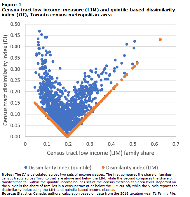
The DI can be interpreted as the proportion of families in each census tract that would have to be shifted across income quantiles, or the LIM cut-off, to match the distribution of the CMA as a whole. This is illustrated in Figure 1 for the Toronto CMA. When calculated using the LIM cut-off, the DI is simply the absolute difference between the share of families in a census tract below or above the LIM cut-off, and that of the CMA. It takes on its minimum value of 0 when the census tract matches Toronto’s 20% share of low-income families and increases to either side by construction (see Figure 1). The census tract with the highest share of families below the LIM cut-off is 63%. To match the CMA level, the incomes of 43% of families would have to be lifted above the LIM cut-off, which is the DI value.
When calculated using quintile-based income classes, finer income breakdowns provide more latitude for sorting families by income across census tracts. Therefore, for census tracts with low shares of families with incomes below the LIM cut-off, the DI values can be quite high, rivalling those census tracts where the share of families below the LIM cut-off is well above 20% (see Figure 1). Hence, while the LIM-based income classes are useful for illustrative purposes, they do not fully capture the scope of income sorting. This raises the question of whether quintile-based classes are sufficiently detailed themselves, which is addressed below.
While the DI is easily interpreted, it cannot be decomposed. That is, it is not possible to determine consistently how families contribute to income mixing within neighbourhoods—by further sorting across dwelling types or across individual apartment buildings—and how this contributes to overall levels of income mixing. The other incoming mixing measures discussed in detail, namely the H-index and D-index, are additively decomposable.
Description for Figure 1
The title of Figure 1 is “Census tract low-income measure (LIM) and quintile-based dissimilarity index (DI), Toronto census metropolitan area.” This figure contains one scatter graph. The values on the x-axis start at 0 and end at 0.7, with graduation marks every 0.1 unit. The values on the y-axis start at 0.00 and end at 0.50, with graduation marks at every 0.05 unit.
The scatter graph illustrates the effects of using more (and different) income classes on the DI. The LIM-based measure increases linearly away from a low of 0 when the share of families below the LIM cut-off matches that of the census metropolitan area at a value of 0.2. It increases to a maximum value of about 0.15 to the left (lower shares of families below the LIM cut-off) and to a maximum of about 0.43 to the right (higher shares of families below the LIM cut-off). When calculated using quintiles to define the income classes, the dissimilarly index is almost always higher than the LIM-based index and exhibits much more variability for a given LIM share. It ranges from a value of 0.15 to 0.45 when the LIM share is near its lowest value of 0.1 and generally declines in value as the LIM share rises to 0.2 at which point the DI ranges from about 0 to 0.2. After that point it generally rises with the LIM share, with a range of values between 0.1 and 0.3 when the LIM share is 0.3. After that, the data points rapidly thin as the LIM share moves towards its maximum value of 0.6 and the quantile-based DI rises to a maximum of about 0.43.
The notes and source of Figure 1 are as follows:
Notes: The DI is calculated across two sets of income classes. The first compares the share of families in census tracts across Toronto that are above and below the LIM, while the second compares the share of families that fall within the quintile income bounds set at the census metropolitan area level. Reported on the x-axis is the share of families in a census tract at or below the LIM cut-off, while the y-axis reports the dissimilarity index using the LIM- and quintile-based income classes.
Source: Statistics Canada, authors’ calculation based on data from the 2016 taxation year T1 Family File.
Information theory index (H-index): For a discrete distribution of income, the entropy of a CMA ( ) or a census tract ( ) within it can be defined as:
The index can be interpreted as a measure of diversity ranging from a value of 0 if all families are in one income quantile ( ) to a maximum value log ( ) if all families are spread evenly across the quantile classes, which, by definition, is the case at the CMA level [ ].Note In turn, entropy ( ) forms the basis for Theil’s information theory index ( ) (Roberto 2016; Theil and Finizza 1971), which, for census tract in CMA , is defined as:
where the CMA-level entropy forms the benchmark distribution against which income mixing at the census tract level is compared. If has the same entropy as , then the index value is 0. However, if the maximum degree of income sorting occurs where all income is concentrated in one quantile, or above or below the LIM cut-off, the value is 1. From Equation (3), the CMA’s level of income mixing can be calculated using census tract family shares as weights:
The higher the level of , the greater the degree of income sorting that is occurring across census tracts.
The H-index is limited in that it is a measure of relative income diversity and is agnostic as to the source of that diversity (Roberto 2016). Consider an instance where 20% of families in a CMA have incomes below the LIM cut-off. A census tract with this proportion will have the same level of entropy ( ) as the CMA, and the H-index will be 0. However, if 80% of families in the census tract had incomes below the LIM cut-off, the H-index would be 0 as well.They are equally diverse relative to the CMA, but their relative income mixes are different (for a fuller discussion, see Roberto [2016]).Note A measure is needed of how different, or divergent, the income distributions are that, like the H-index, can be decomposed.
Divergence index (D-index): The D-index for a census tract in a CMA is defined as (Roberto 2016)Note :
Rather than comparing a summary of the income distributions, the D-index compares individual census tract income classes with CMA income classes. As with the H-index, CMA-level income divergence is the sum of census tract divergence, , weighted by its share of CMA families:
Regarding interpretation, if the income distribution of census tract matches that of the CMA, , then = 0. Unlike the H-index, there is no upper bound defined for the D-index. This comes with the benefit that the divergence between the income mixes at the CMA and census tract levels is explicitly taken into account.
As Roberto (2016) notes, the D-index measures the degree of “surprise.” In this context, it measures how unusual it would be to observe such a degree of divergence between the income distribution at the census-tract level compared with that at the CMA level. If, as in the example above, 80% of families in a census tract have incomes below the LIM cut-off, while only 20% of families at the CMA level were low income, there would be surprise in the degree of sorting on income and with the expectation of a positive index value ( = 1.2, using ).
Figure 2 (a) illustrates the relationship between the D-index and H-index using LIM-based income classes calculated across census tracts in Toronto. When matching the CMA-level share of families below the LIM cut-off, both indices take on a value of 0. However, when they move away from this point, they take on different values. The H-index turns negative when census tracts with LIM shares rise to a minimum value when the LIM share is 50%, as this represents an even more diverse income composition where families above and below the LIM cut-off are equally represented. Furthermore, the relationship between the H-index and the LIM share is non-monotonic, eventually rising and crossing the x-axis when 80% of families fall below the LIM cut-off. However, the D-index progresses upward from its minimum, capturing how surprising it is to observe the share of families in a census tract below the LIM cut-off relative to that of the CMA. It is on this basis that this paper’s preference for the D-index rests.Note
The downside of the D-index is that it lacks an upper bound and it is not as easily interpretable as the DI. One way to address this problem is to relate the two indices. Figure 2 (b) plots the D-index on the DI using quintile-based income classes. Both tell similar stories, with a non-linear relationship that is strong enough that the D-index can be described in terms of its related DI values with some confidence. A D-index value of 0.05, for instance, implies that about 15% of families would have to be shifted across income classes to match the CMA income mix. The strong association between the indices means the upcoming focus on the D-index results in little loss of generality.
Two questions remain. The first is whether the D-index is sensitive to the granularity of the income classes used to measure income mixing. One concern is that using overly aggregate categories results in a considerable loss of information (Reardon and Bischoff 2011). To test this, the D-index was calculated for Toronto, defining income classes using percentiles rather than quintiles. The cross-census-tract correlation between the percentile- and quintile-based D-index was very high, at 0.93. Hence, relatively little information is lost when quintiles are used to measure income mixing. The second question is how the D-index can also take into account the effects of sorting families across dwelling types and, given the data, individual buildings, which is dealt with next.

4.2 Decomposing income mixing
While the degree of sorting of families across census tracts (neighbourhoods) is of considerable interest, an additional key objective is to measure the extent of income mixing across dwelling types and within multi-unit apartment buildings. Adding this dimension to this paper’s definition of neighbourhoods raises two related questions:
- How much of the income mixing in a census tract stems from
sorting on income across dwelling types?
A census tract might appear to be diverse, but a significant portion of that diversity may come from sorting on income between identified apartments ( ) and other dwelling types ( ). Large multi-unit apartments can be islands of low-income families set within a sea of higher-income single-family homes. If neighbourhood-based externalities are highly localized (e.g., crime), the relative isolation of low-income families in large apartment blocks may matter. - How much of income mixing is due to sorting on income
across apartment buildings?
The income mixing observed in apartment buildings as a group may stem from the sorting of low- and high-income families across buildings (e.g., between expensive high-rise condo towers and lower-cost rental apartment buildings).
In mathematical terms, the decomposition is developed in steps. The first step is to decompose census tract income mixing, after taking into account sorting across dwelling types. Next, the decomposition is expanded to include sorting across individual buildings. The D-index at the census tract dwelling-type level ( ) aggregated up to the CMA level is given by:
where . In turn, this can be decomposed into between-census-tract divergence and within-census-tract divergence across dwelling types, with the latter given by:
In this instance, the reference income distribution is at the census-tract level ( ) and provides a means to measure how much each census tract’s income mix varies across dwelling types. The total level of income divergence is the sum of the between-census-tract income divergence (Equation [6]) and the family-weighted average of the within-census-tract divergence across dwelling types:
Therefore, for the CMA as a whole, the degree of income divergence stemming from sorting families across census tracts and across dwelling types within census tracts can be measured.
By the same token, the effect of sorting across apartment buildings within the apartment dwelling type can be measured, resulting in a CMA measure of census-tract dwelling type apartment-building divergence:
where . From this, the D-index can be subdivided into subcomponents in an analogous fashion to (9):
where within-census-tract dwelling type divergence across buildings is given by
Finally, substituting (9) into (11) results in the following complete decomposition across all levels:
At the CMA level, the first term measures the contribution of sorting on income across census tracts to income divergence—that is, the degree to which poorer and richer families are sorting into neighbourhoods with similar income levels. The second term measures the effect of sorting across dwelling types within census tracts. This takes into account the possibility that there could be minimal sorting on income across neighbourhoods, but considerable sorting on income across dwelling types, with possibly the poorer families concentrating in large apartment blocks and the remaining higher-income families living in other types of dwellings. The third term measures the sorting of families on income across apartment buildings. This captures the possibility that sorting may be occurring at a fine level, across buildings in this instance. A similar decomposition can also be done for individual census tracts, such that the contribution of sorting across dwelling types, and individual apartment buildings at the census-tract level, can be taken into account.
Additional income mixing measures: Several other income mixing measures that are continuous in nature were also considered, such as the Neighbourhood Sorting Index (Jargowsky 1996) and the Centile Gap Index (Watson 2009). Theoretically, less information is lost through continuous measures (Reardon and Bischoff 2011). However, in practice, these measures do not appear to provide an advantage over income mixing measures that are based on the discretized income distributions described previously.
First, as previously noted, the correlation between the census tract D-index calculated across quintiles and percentiles is 0.93 for Toronto.Note Hence, relatively little information is lost moving from this near-continuous measure to more aggregate quintiles. Second, continuous measures are more sensitive to the extremes of the income distribution. This would be particularly problematic for census tracts with small populations and, especially, individual apartment buildings. Third, unlike the D-index, these measures are less amenable to decomposition across sub-classes, which is a major advantage when working with data classified by census tract, dwelling type and individual building. Lastly, income mixing implies the combination of families across income strata, which implies a discrete set of income classes. It is not necessary to describe income distributions in a continuous fashion to develop a measure that is consistent with the concept.
5 Income mixing across census metropolitan areas
This section describes income mixing across CMAs. It progresses by examining the variation in income across census tracts, dwelling types and buildings within CMAs. This is followed by a description of income mixing across CMAs using the D-index, and its decomposition into contributions from sorting on income across dwelling types and apartment buildings within census tracts.
5.1 Income across census tracts, dwelling types and buildings
To provide some basic context, Table 2 presents average family income levels, adjusted for family size, across census tracts for selected CMAs. Average census tract incomes are highest in Calgary and Edmonton, and lowest in Montréal and the city of Québec. The degree of variation in incomes across census tracts is at issue. This is captured by the ratio of average census tract incomes across a set of percentile ranks. The ratio of incomes ranked at the 95th percentile to those at the 5th percentile provides a measure of the spread of census tract mean incomes. All the CMAs reported have a ratio of 2 or more, with Toronto the highest at 2.9. This is broadly consistent with earlier census-based findings (Chen, Myles and Picot 2012). The ratios of the 95th to the 50th and the 50th to the 5th percentiles provide an indication of whether the spread is coming from the upper or lower ends of the census tract income distribution. The ratios are quite similar for most of the CMAs reported, which indicates that a small selection of very high- or very low-income census tracts is not driving the overall spread.
| Census metropolitan areas | Mean census tract income | 95th to 5th percentile | 95th to 50th percentile | 50th to 5th percentile |
|---|---|---|---|---|
| dollars | ratio | |||
| Halifax | 43,900 | 2.0 | 1.4 | 1.4 |
| Québec | 42,400 | 2.0 | 1.4 | 1.4 |
| Montréal | 41,400 | 2.4 | 1.6 | 1.5 |
| Ottawa–Gatineau | 50,000 | 2.5 | 1.4 | 1.6 |
| Toronto | 47,900 | 2.9 | 1.9 | 1.5 |
| Winnipeg | 42,700 | 2.7 | 1.6 | 1.7 |
| Calgary | 56,900 | 2.5 | 1.6 | 1.6 |
| Edmonton | 52,000 | 2.2 | 1.5 | 1.4 |
| Vancouver | 46,200 | 2.2 | 1.5 | 1.4 |
|
Note: Percentile ratios are based on the mean adjusted after-tax family income, measured across census tracts within each census metropolitan area. Source: Statistics Canada, authors’ calculation based on data from the 2016 taxation year T1 Family File. |
||||
As noted above, while families may sort on income across census tracts, they may also sort across dwelling types and across individual apartment buildings within census tracts. Whether these types of sorting matter depends on how much variation there is on incomes across dwelling types and buildings.
Table 3 presents the average ratio of incomes of families in identified apartments relative to other dwelling types across census tracts and demonstrates how much variation there is across census tracts by presenting their percentile ranks. On average, incomes of families living in apartments across census tracts are about 80% of those of families living in other types of dwellings. This is consistent across the CMAs reported, with the exception of Vancouver, where the incomes of families living in apartments are 95% of those of families living in other types of dwellings.
Across census tracts, there is considerable variation in the relative incomes of families living in apartments and other dwelling types. In some census tracts, incomes of families in apartments are far lower than incomes of families living in other types of dwellings, while in others the opposite is true, albeit not to quite the same extent. For instance, in Toronto, the ratio ranges across census tracts from 0.44 in the 5th percentile to 1.20 in the 95th. Not all families in apartments, which may be rental or condo apartments, earn less than their neighbours in other dwelling types.
| Census metropolitan areas | Mean | Percentiles of mean income ratios across census tracts | ||||
|---|---|---|---|---|---|---|
| 5th | 25th | 50th | 75th | 95th | ||
| ratio | ||||||
| Halifax | 0.81 | 0.47 | 0.66 | 0.78 | 0.90 | 1.39 |
| Québec | 0.81 | 0.50 | 0.62 | 0.81 | 0.93 | 1.16 |
| Montréal | 0.83 | 0.43 | 0.61 | 0.77 | 0.96 | 1.43 |
| Ottawa–Gatineau | 0.81 | 0.44 | 0.62 | 0.77 | 0.96 | 1.28 |
| Toronto | 0.79 | 0.44 | 0.63 | 0.76 | 0.91 | 1.20 |
| Winnipeg | 0.78 | 0.47 | 0.66 | 0.77 | 0.86 | 1.08 |
| Calgary | 0.81 | 0.47 | 0.68 | 0.80 | 0.92 | 1.10 |
| Edmonton | 0.82 | 0.57 | 0.68 | 0.81 | 0.93 | 1.13 |
| Vancouver | 0.95 | 0.58 | 0.84 | 0.95 | 1.07 | 1.27 |
|
Note: Percentiles are based on the mean adjusted after-tax income of families living in apartment buildings relative to other dwelling types, measured across census tracts within each census metropolitan area. Source: Statistics Canada, authors’ calculation based on data from the 2016 taxation year T1 Family File. |
||||||
Finally, Table 4 reports the variation in average apartment building family incomes across CMAs. Once again, there is considerable variation across buildings, with the ratio of the 95th to the 5th percentile in Toronto being close to 4. This is greater than the variation observed in average incomes across Toronto’s census tracts. Like sorting across dwelling types, sorting on income across buildings within census tracts may influence overall levels of income mixing. It is to this question, and to a broader overview of the level of income mixing across CMAs, that the discussion now turns.
| Census metropolitan areas | 95th to 5th percentile | 95th to 50th percentile | 75th to 25th percentile | 50th to 5th percentile |
|---|---|---|---|---|
| ratio | ||||
| Halifax | 3.4 | 1.8 | 1.6 | 1.9 |
| Québec | 3.5 | 1.7 | 1.6 | 2.0 |
| Montréal | 4.5 | 2.5 | 1.9 | 1.8 |
| Ottawa–Gatineau | 4.4 | 2.2 | 1.9 | 2.0 |
| Toronto | 3.9 | 2.2 | 1.7 | 1.7 |
| Winnipeg | 4.1 | 1.8 | 1.6 | 2.3 |
| Calgary | 3.6 | 2.0 | 1.5 | 1.8 |
| Edmonton | 3.0 | 1.8 | 1.5 | 1.7 |
| Vancouver | 3.4 | 1.7 | 1.5 | 2.0 |
|
Note: Percentiles are based on the mean adjusted after-tax income of families living in apartment buildings in selected census metropolitan areas. Source: Statistics Canada, authors’ calculation based on data from the 2016 taxation year T1 Family File. |
||||
5.2 Indices of income mixing
This section describes the income mix of CMAs using the D-index. Although the DI could be used for comparison, as previously noted, it is strongly associated with the D-index (see Figure 2 [b]). Therefore, the discussion from this point forward concentrates on the D-index, for the sake of brevity.Note
To provide further context on the variation in income mixing across CMAs, Figure 3 presents box plots of census-tract-level D-index values ( ) across the same selection of CMAs used above. The box plots illustrate the degree of variability in income mixing across census tracts within CMAs. The bottoms and tops of the boxes are the 25th and 75th percentiles. Therefore, the lengths of the boxes represent the interquartile range.
The lines intersecting the boxes indicate the median D-index values within a CMA. The ends of the “whiskers” represent the lowest and highest datum within up to 1.5 times the interquartile range from the first and third quartiles. In essence, the whiskers help to illustrate a reasonable range of values, though they do not preclude extreme values that lie outside the top and bottom whiskers.
Across the CMAs reported, the median census tract D-index is around the same value (0.025), but the range of values varies considerably—the interquartile range for Winnipeg is about twice that of Vancouver, with Winnipeg’s upper quartile at about 0.08, and Vancouver’s at about 0.04. The whiskers indicate that, across all CMAs, there are low values near 0 (income mixes nearly matching the census tract’s CMA) and high values ranging from a little under 0.1 to about 0.175 across the selected CMAs. These correspond roughly to the 95th percentiles of the CMAs’ respective D-index distributions. No census tracts have a D-index above 0.9 across all CMAs.

Description for Figure 3
The title of Figure 3 is “Box plot of D-index across census tracts, selected census metropolitan areas.”
The y-axis plots the D-index box plot values of the selected CMAs. The values range from 0 to 0.2, with graduations at every 0.05 unit. Reported along the x-axis are the box plots of the nine selected census metropolitan areas (CMAs), which are reported to give readers an overview of the variability of the D-index within and across CMAs.
The note and source for Figure 3 are as follows:
Note: D-index: divergence index.
Source: Statistics Canada, authors’ calculation based on data from the 2016 taxation year T1 Family File.
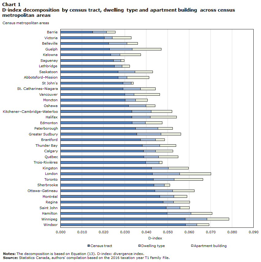
The degree to which sorting on income across dwelling types and buildings within census tracts also influences income mixing is at issue. Chart 1 presents the decomposition of the D-index across CMAs, as described in Equation (13). The height of the bars measures the CMA-level D-index values and allows for sorting on income across census tracts and within census tracts across dwelling types and buildings. CMAs are ordered based on the contribution of sorting on income across census tracts ( ), which makes the largest contribution across all CMAs.
Based on this ranking, the Windsor, Winnipeg and Hamilton CMAs have, on average, the neighbourhoods with the least income mixing, while neighbourhoods in Belleville, Victoria and Barrie have the most. Sorting on dwelling type and individual apartment buildings adds roughly one-third to the overall D-index levels, but with considerable variation across CMAs. Importantly, taking into account sorting on dwelling type and buildings would substantially change the rankings. For instance, Toronto and London would move up the rankings from 9th and 10th to 5th and 4th, respectively.
Data table for Chart 1
| Census metropolitan areas | Census tract | Dwelling type | Apartment building |
|---|---|---|---|
| D-index | |||
| Barrie | 0.015 | 0.007 | 0.004 |
| Victoria | 0.020 | 0.004 | 0.009 |
| Belleville | 0.022 | 0.008 | 0.005 |
| Guelph | 0.023 | 0.011 | 0.014 |
| Kelowna | 0.023 | 0.004 | 0.010 |
| Saguenay | 0.025 | 0.003 | 0.002 |
| Lethbridge | 0.025 | 0.004 | 0.004 |
| Saskatoon | 0.027 | 0.008 | 0.008 |
| Abbotsford–Mission | 0.027 | 0.004 | 0.010 |
| St John's | 0.029 | 0.004 | 0.001 |
| St. Catharines–Niagara | 0.029 | 0.008 | 0.007 |
| Vancouver | 0.030 | 0.004 | 0.012 |
| Moncton | 0.030 | 0.005 | 0.005 |
| Oshawa | 0.032 | 0.008 | 0.004 |
| Kitchener–Cambridge–Waterloo | 0.033 | 0.009 | 0.010 |
| Halifax | 0.033 | 0.009 | 0.012 |
| Edmonton | 0.033 | 0.006 | 0.008 |
| Peterborough | 0.035 | 0.010 | 0.007 |
| Greater Sudbury | 0.036 | 0.011 | 0.009 |
| Brantford | 0.037 | 0.007 | 0.004 |
| Thunder Bay | 0.038 | 0.008 | 0.008 |
| Calgary | 0.039 | 0.006 | 0.008 |
| Québec | 0.039 | 0.007 | 0.009 |
| Trois-Rivières | 0.040 | 0.006 | 0.001 |
| Kingston | 0.042 | 0.008 | 0.009 |
| London | 0.043 | 0.013 | 0.015 |
| Toronto | 0.043 | 0.010 | 0.013 |
| Sherbrooke | 0.044 | 0.005 | 0.003 |
| Ottawa–Gatineau | 0.044 | 0.008 | 0.010 |
| Montréal | 0.046 | 0.007 | 0.006 |
| Regina | 0.048 | 0.005 | 0.008 |
| Saint John | 0.049 | 0.006 | 0.005 |
| Hamilton | 0.050 | 0.011 | 0.010 |
| Winnipeg | 0.058 | 0.010 | 0.010 |
| Windsor | 0.058 | 0.005 | 0.006 |
|
Notes: The decomposition is based on Equation (13). D-index: divergence index. Source: Statistics Canada, authors' compilation based on the 2016 taxation year T1 Family File. |
|||
6 Conclusions
This paper outlines several income mixing measures. Priority was given to measures that are easily interpreted and that can be decomposed across levels of analysis, namely neighbourhoods, dwelling types and individual buildings. The latter is particularly important because it provides a means to estimate and understand income mixing using units of analysis sufficiently detailed to be relevant to housing policy. Indeed, the decomposition proved powerful, illustrating how all three components are important and demonstrating their variable effects across census metropolitan areas.
A number of additional steps should be taken to further improve the quality and utility of the income mixing measures presented here. Perhaps most promising is the planned linkage of the T1 Family File and the Address Register. This linkage provides a means to identify more precisely the location of taxfilers. This will allow for income mixing to be measured at the dissemination-area level (or below), and would further increase the precision of analytical estimates at more detailed levels of geography. Many more steps might be undertaken, including testing the statistical significance of the differences in income mixing across units and determining the spatial association of the income mixing measures (i.e., whether there is a correlation with neighbouring units).
Appendix: Inequality measures
It is important to distinguish between income mixing within neighbourhoods and inequality across individuals and neighbourhoods. Income inequality at the individual (or family) level is a necessary condition for the presence of between-neighbourhood inequality and income mixing within neighbourhoods (Reardon and Bischoff 2011). Sorting on income across neighbourhoods will result in higher levels of between-neighbourhood inequality and lower levels of income mixing within neighbourhoods.Note Indeed, Chen, Myles and Picot (2012) showed that, across eight CMAs from 1980 to 2005, income inequality has been rising, as has the level of inequality across neighbourhoods (i.e., census tracts). This is associated with higher levels of income segregation (see also Myles, Pyper and Picot 2000; Bolton and Breau 2012). Notably, Fong (2017) showed that, although income inequality in Canada grew through the 1980s and 1990s, it was largely a metropolitan phenomenon. This reinforces this paper’s focus on income mixing measures across CMAs. In the non-metropolitan (non-CMA) parts of Canada, income inequality on an after-tax basis has not risen since the 1970s.Note
The focus of this paper’s income mixing measures has been on distributional measures that use the census tract as their reference distribution, which better addresses this program of work’s specific objectives. Nevertheless, income mixing is predicated on the presence of income inequality and, at some point, it may be useful to measure inequality as well. There are many income inequality measures, including the Gini index and various forms of the Theil index. The Theil index, which can be derived from a special form of the D-index (Roberto 2016), is additive in nature, and so it is able to measure the contribution of neighbourhood inequality to metropolitan-level inequality. At the neighbourhood level, the Theil index takes the following form:
and
where is the population of families in geographic unit , is the income of family and is the average family income in . and are different versions of the Theil index—where the former is more sensitive to differences in income share at the top of the income distribution, and the latter is more sensitive to differences in income share at the lower end of the income distribution.Note
As a note of caution, Wolfson (1997) argues that the Theil index can be problematic because it is sensitive to very small values, which can result in spurious results. Therefore, the sensitivity of results to this effect would have to be tested, or other alternatives would have to be tested.
References
Baldwin, J., M. Frenette, A. Lafrance, and P. Piraino. 2011. Income Adequacy in Retirement: Accounting for the Annuitized Value of Wealth in Canada. Economic Analysis Research Paper Series, no. 74. Statistics Canada Catalogue no. 11F0027M. Ottawa: Statistics Canada.
Bolton, K., and S. Breau. 2012. “Growing unequal? Changes in the distribution of earnings across Canadian cities.” Urban Studies 49 (6): 1377–1396.
Breau, S., M. Shin, and N. Burkhart. 2018. “Pulling apart: New perspectives on the spatial dimensions of neighbourhood income disparities in Canadian cities.” Journal of Geographical Systems 20 (1): 1–25.
Brown, W.M., and A. Lafrance. 2010. Incomes from Owner-occupied Housing for Working-age and Retirement-age Canadians, 1969 to 2006. Economic Analysis Research Paper Series, no. 66. Statistics Canada Catalogue no. 11F0027M. Ottawa: Statistics Canada.
Brown, W.M., A. Lafrance, and F. Hou. 2010. Incomes of Retirement-age and Working-age Canadians: Accounting for Home Ownership. Economic Analysis Research Paper Series, no. 64. Statistics Canada Catalogue no. 11F0027M. Ottawa: Statistics Canada.
Chen, W.-H., J. Myles, and G. Picot. 2012. “Why have poorer neighbourhoods stagnated economically while the richer have flourished? Neighbourhood income inequality in Canadian cities.” Urban Studies 49 (4): 877–896.
Duncan, O.D., and B. Duncan. 1955. “Residential distribution and occupational stratification.” American Journal of Sociology 60 (5): 493–503.
Fong, F. 2017. Income Inequality in Canada: The Urban Gap. Technical report. Toronto: Chartered Professional Accountants of Canada. (accessed July 11, 2019).
Jargowsky, P.A. 1996. “Take the money and run: Economic segregation in U.S. metropolitan areas.” American Sociological Review 61 (6): 984–998.
Kullback, S. 1987. “Letter to the editor: The Kullback-Leibler distance.” American Statistician 41 (4): 340–341.
Myles, J., W. Pyper, and W. Picot. 2000. Neighbourhood Inequality in Canadian Cities. Analytical Studies Branch Research Paper Series, no. 160. Statistics Canada Catalogue no. 11F0019M. Ottawa: Statistics Canada.
Oreopoulos, P. 2008. “Neighbourhood effects in Canada: A critique.” Canadian Public Policy 34 (2): 237–258.
Pinard, D. 2018. Methodology Changes: Census Family Low Income Measure Based on the T1 Family File. Income Research Paper Series, no 1. Statistics Canada Catalogue no. 75F0002M. Ottawa: Statistics Canada.
Reardon, S.F., and K. Bischoff. 2011. “Income inequality and income segregation.” American Journal of Sociology 116 (4): 1092–1153.
Roberto, E. 2016. The Divergence Index: A Decomposable Measure of Segregation and Inequality. Preprint, last revised December 5, 2016. (accessed July 11, 2019).
Statistics Canada. 2018. “Annual Income Estimates for Census Families and Individuals (T1 Family File): Detailed information for 2016.
Statistics Canada. 2019a. “Census tract (CT).” Dictionary, Census of Population, 2016. Last modified January 3, 2019. (accessed October 18, 2019).
Statistics Canada. 2019b. “Census family.” Last modified August 20, 2019. (accessed October 21, 2019).
Strelch, P. 2016. Assessment of Income Mixed Housing Models that Support Affordable Housing Viability. Ottawa: Canada Mortgage and Housing Corporation.
Theil, H., and A.J. Finizza. 1971. “A note on the measurement of racial integration of schools by means of informational concepts.” Journal of Mathematical Sociology 1 (2): 187–193.
Walks, A. 2013. Income Inequality and Polarization in Canada’s Cities: An Examination and New Form of Measurement. Research Paper 227. Toronto: Cities Centre, University of Toronto.
Watson, T. 2009. “Inequality and the measurement of residential segregation by income in American neighborhoods.” Review of Income and Wealth 55 (3): 820–844.
Wikipedia. 2019. “Theil index.” Wikipedia Foundation. Last modified October 19, 2019. (accessed October 21, 2019).
Wolfson, M.C. 1997. “Divergent inequalities: Theory and empirical results.” Review of Income and Wealth 43 (4): 401–421.
- Date modified: