Findings

View the most recent version.

The Canadian Community Health Survey (CCHS) consists of two cross-sectional sample surveys. The .1 cycle collects general health information from more than 120 health regions, while the .2 cycle focuses on specific health topics and collects data for estimation at the provincial level.

Despite large sample sizes, a single CCHS cycle may not meet users’ needs. For instance, researchers may be interested in studying a rare population defined by detailed geography or by relatively rare socio-demographic or health characteristics. Because a single cycle may yield few observations for such a population, combining cycles may be considered. For example, this option was used by Tremblay et al.¹ in an examination of the relationship between body mass index and ethnicity, and by Tjepkema² in a study of health care use among gay, lesbian and bisexual Canadians.

The possibility of combining cycles exists because data for the same characteristics have generally been collected in all .1 cycles, and some of the same information is collected in .2 cycles. Nonetheless, as the CCHS has evolved, differences have emerged from cycle to cycle that may mean combining cycles is not feasible, or if still possible, may affect the results, depending on the analytical objectives of the study.

This article explains methods of combining CCHS cycles and offers guidelines for interpreting the results. Although the information pertains specifically to the CCHS, many of the issues have broader applicability. A case study illustrates the methods and shows that satisfactory estimates can be produced from combined cycles.

Starting in 2007, the CCHS implemented continuous collection with the intention of producing annual files as well as two-year combined files. This introduces different “period estimates,” which will be the topic of a related article. This article focuses on the methodology and considerations for combining past cycles of the CCHS. 

An evolving survey

The CCHS was not designed as a rolling sample,^3, 4 expressly constructed to allow the different samples collected over time to be combined. Consequently, combining should be undertaken only after it has been determined that the estimates from a single cycle do not meet analytical needs, and also, that the combined results will be relevant and interpretable.

Since its inception in 2000/2001, the CCHS has evolved. Consequently, the estimates derived from different cycles may not be comparable. To determine if combining cycles is feasible, changes in questionnaire content, survey coverage, geography, and mode of collection must be considered.

Changes in content

The CCHS questionnaire has undergone continual modification, including the introduction of new modules and removal of old ones. When content modifications are substantial, variable names usually change. Nonetheless, the same variable name does not necessarily indicate that exactly the same question was asked, so the wording of questions should be verified before cycles are combined. Users can consult CCHS documentation, notably the data dictionaries and questionnaires available from Statistics Canada’s website (surveys and statistical programs within Definitions, Data Sources and Methods). Revisions to question wording, module structure, and response categories may mean that combining is not appropriate.

Changes in coverage

The populations targeted by certain modules of the CCHS questionnaire may differ from cycle to cycle. The most obvious example is the optional content that health regions/provinces can choose. As a result, the modules administered to the residents of a particular area in one cycle may be asked of the residents of an entirely different area in the next.

Another possibility is a change in the target population of a module. For instance, in cycle 1.1, the sexual behaviour module was asked of people aged 15 to 59, but in cycle 2.1, the target age group was narrowed to 15 to 49.

Changes in geography

The data file for each CCHS cycle contains geography coding and identifiers for the health regions as they were when the data were disseminated. However, health regions can change from one cycle to another. While these may be as minor as changes in names or codes, it is also possible for boundaries to be redrawn. If this has occurred, the files must be updated to a common geography (usually the most recent) before cycles can be combined. More information about boundary changes is available in the Internet publication, Health Indicators (health regions and peer group section, health region changes subsection). If updated health region boundaries are required, correspondence files providing the relationship between Dissemination Areas (DA) or Enumeration Areas (EA) and the health regions for a given reference period are available in the Internet publication, Health Regions: Boundaries and correspondence with census geography.

Changes in mode

The “mode effect” is the impact the method of collection has on the way respondents answer survey questions. CCHS interviews are conducted both by telephone and in person. The information that respondents provide can differ depending on the mode used for their interview. A 2004 study⁵ found that several CCHS variables are susceptible to the mode effect, including, but not limited to, height and weight, physical activity, contact with doctors, and unmet health care needs. 

To secure consistent estimates, efforts are made to maintain the same mix of telephone and personal interviews from one cycle to the next.  However, large supplementary additions to the survey (buy-in samples) can affect the telephone/personal interview balance, because these supplementary interviews are usually conducted by telephone. For cycle 1.1, the proportion of telephone interviews was quite low, a factor that should be recognized when considering combining that cycle with others.

Combining different surveys

For the reasons outlined above, the results of different cross-sectional health surveys may not be comparable, and in most situations, should not be combined. Therefore, it is recommended that the regional component of the CCHS (.1 cycles) not be combined with the provincial components (.2 cycles – Mental Health (2002) and Nutrition (2004)).

An evolving population

The feasibility of combining CCHS cycles derives from the fact that if random samples are taken from a population, the accumulated samples can be considered as one large random sample from the same population. However, if the population changes significantly between cycles, the samples cannot be treated as though they came from the same population. In the case of the CCHS, the samples for the successive cycles are drawn from an evolving population. Consequently, the combined sample is not necessarily representative of any of the populations represented by one cycle alone, but rather, the combined population.

Differences that emerge from cycle to cycle may stem from the reasons mentioned above—changes in the questionnaire, coverage and collection mode—or from sampling variability. However, changes from one cycle to another may reflect actual changes in the parameter under study. In such situations, combining cycles is still possible, but interpretation of the results requires an understanding of the effect of the time periods covered by the combined sample estimate. It is also important to be aware that, when combined in a single estimate, such trends will be obscured.

Methods for combining

Methods for combining data from different surveys can be divided into two broad categories: the separate approach and the pooled approach. The separate approach employs composite estimation techniques, whereby estimates are calculated for each survey separately and then combined. The pooled approach combines sample data at the micro-data level, and the resulting dataset is treated as if it is a sample from one population.

The separate approach

The separate approach creates an average of estimates calculated from the different CCHS cycles. The advantage is that, with some assumptions, the combined result is easy to interpret. As well, an average can be calculated from existing tables, which makes the approach appealing to users of the Public Use Microdata Files (PUMFs) and to those who rely on existing tables of estimates.

The disadvantage of the separate approach is that it can be cumbersome. If the required estimates are not published or do not include the variances, estimates must be calculated from each survey separately before being integrated. PUMF users will be limited by the information contained on the PUMF, and users relying on tables will have to gain access to the microdata. If many estimates are needed, the process is time-consuming.

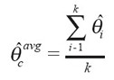
In the case of the CCHS, estimates of a population parameter θ (which can be any statistic such as a mean, total or ratio) can be calculated separately for each cycle, , where k is the number of cycles available. A simple average can then be calculated as:

For variance to be estimated relatively easily, the samples must be independent, which is true for most CCHS cycles. The exceptions are 2.1 and 2.2, where cycle 2.1 respondents were used as a frame for cycle 2.2. Therefore, cycles 2.1 and 2.2 cannot be easily combined with the separate approach.

Based on the assumption of independence between the cycles, an estimate of the variance of the simple average of the three .1 cycles can be calculated as:

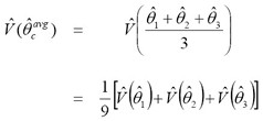
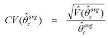
It is evident that the estimated variance of the average of the three cycles is roughly one-third of the estimated variance of an estimate from one cycle alone. Standard errors can be calculated by taking the square-root of the variance, and estimates of the CV can be calculated as:

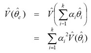
In some instances, it may be desirable to estimate a weighted average rather than the simple average, with more weight given to one estimate than another. Assuming that a researcher is interested in estimating for the same parameter θ as described with the simple average, separate estimates can be calculated, and a composite estimate or a weighted average can then be calculated as:

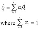
If each estimate is an unbiased estimate of θ, then will also be unbiased, for any choices of α_i. That is, if each cycle correctly estimates the same constant statistic for the same population, the combined result will correctly estimate the same statistic.

Depending on the analysis, there are several choices for α_i. Some choices include an increasing weight function with more weight given to more current cycles, or a weight function based on variances, which results in a more efficient estimate of the population parameter (that is, lower variance). More information about these methods is available in Chu, Brick and Kalton⁶ and Korn and Graubard.⁷

Once the composite estimate has been computed using the appropriate value of i, an estimate of the variance can be calculated as a function of the original variances, and standard errors and CVs can be estimated. Assuming the cycles are independent, the variance can be estimated as:

For the separate approach to yield an unbiased estimate of a population parameter, the estimates being combined must each be unbiased estimates of the same population parameter. As noted earlier, this is problematic for the CCHS, the purpose of which is to measure the characteristics of an evolving population at different points in time. Because the assumption of a constant statistic is questionable, thereby making a weighted average difficult to interpret, it is recommended that users interested in the separate approach employ the simple average, where this assumption is not required, and the result is easier to interpret.

The pooled approach

The pooled approach consists of combining different CCHS cycles at the micro-data level to obtain a dataset that can be analysed as a single sample from a population. The pooled approach is an attractive option because of the power of the increased sample size, and because, once combined, it is not necessary to return to the individual datasets.

The disadvantages are that more technical expertise in the manipulation of data files is required, and it is not an option for users who do not have access to the microdata files. PUMF users are able to calculate an estimate using the pooled approach, but cannot calculate the variance because CV tables are not available for the combined data file.

In its most basic form, pooling involves taking the individual data files with the corresponding weights and using a simple merge or set statement in SAS to create one data file. At the same time, the bootstrap weight files must be combined for variance estimation. Once these files are created, the resulting data file and bootstrap weight file can be treated as if it was one sample from one population. Estimates of rates and proportions, as well as statistical models, can be created with the files and any statistical program capable of estimating variances using the bootstrap method, such as Statistics Canada’s Bootvar program.

The approach described above may not be appropriate for estimating totals. For example, to estimate the number of diabetes cases from two independent surveys of a common population, it is not possible to sum the sample weights from both surveys for respondents with diabetes—this would overestimate the total by a factor of two.⁷ An option is to rescale the original sampling weights w_i by the factor α_i to represent the population of interest, as was done with the separate approach.

There are several choices of α_i.⁸ Because the assumption that each CCHS cycle can be used to estimate the same population parameter is questionable, it is recommended that weights be scaled by a constant factor, α_i=1/k. If two cycles are combined, this means that α=0.5; in the case of three cycles, α=0.33. The resulting estimates can be interpreted as representing the characteristics of the average population (or a period estimate), which covers the combined time periods of the individual cycles. This does not require the assumption that each cycle estimates the same parameter.

It is not always necessary to adjust the weights when pooling the data. When weights are adjusted, the assumption is that they are being adjusted to properly represent a population. The problem is that when weights from different time periods are combined, the resulting weights do not represent the current population, but rather, an average population that does not exist. Consequently, creating totals with a combined file may not be appropriate, whether or not the weights are adjusted. On the other hand, ratios, proportions and means can be regarded as useful statistics when considered as period estimates. For these types of statistics, the results using the original weights or the weights that have been adjusted using a common α_i=1/k will give the same result. This also holds for regression parameters, where weights are used in the model in order to take the survey design into account rather than to make estimates for some finite population.

One of the main applications of the pooled approach is in complex analysis using regression models.^1, 2 With the increased sample size available from combined data, more detailed regression models can be studied. As well, the cycle/time effect can be considered in the model, and if significant, controlled. Other factors such as the mode effect can also be considered/controlled in such models, thereby making it possible to combine results from different cycles that would otherwise not be comparable.

Comparing approaches

The separate approach and the pooled approach do not always yield the same estimate. As an illustration, the separate approach of taking a simple average of two ratios, a/b and c/d, is not equal to the pooled approach, where a period estimate is calculated. This is because, generally speaking

(a/b + c/d) ≠ (a + c)/(b + d)

Therefore, while both methods are valid, the choice depends on the goal of the analysis. Using a Canada estimate as an example, some researchers may choose to study the average of provincial estimates, which gives equal weight to each province (separate approach), while others are interested in the national estimate (pooled approach), which is influenced more by larger provinces.

For ratios such as a proportion, the two approaches will generally yield the same results as long as the parameter being estimated remains constant between the two occurrences, or the populations remain unchanged. For statistics such as regression parameters, it may be preferable to use a pooled approach to calculate the parameters instead of taking an average of the regression parameters calculated from the different cycles.

The Durham project

In 2007, the Durham (Ontario) health unit proposed producing a report on the health of Durham’s adolescents, using combined CCHS data. The Adolescent Health Snapshot would target the 12-to-19 age group, and when possible, ages 12 to 14 and 15 to 19 separately. Based on combined CCHS data, Durham rates would be compared with provincial rates to reveal differences that were not evident from one cycle alone.

The variables of interest (typically, low-prevalence characteristics) were:

• daily smokers
• daily and occasional smokers
• current alcohol drinkers
• heavy drinkers
• sexual activity
• level of physical activity
• physical inactivity
• fruit and vegetable consumption
• use of protective gear ( helmets while biking) 
• overweight and obesity (youth body mass index - BMI)

After initial analysis to ensure that comparable data were available from more than one CCHS cycle, two variables were dropped:

• protective equipment, because of questionnaire changes across cycles 
• BMI, because the derived variable created for cycle 3.1 was not available for cycles 1.1 and 2.1.

Several other potential variables could not be included because they had not been selected consistently as optional content by Durham region: suicidal thoughts, food insecurity, and illicit drug use. (An ancillary benefit of this project was that the value of combining cycles became evident and may influence regions’ selection of optional content in the future.)

The daily smokers variable illustrates the process of combining cycles. For any analysis, it is recommended that there be at least 10 observations with the characteristic under study before an estimate is calculated. Even with combined data, analysis of the 12-to-14 age group was not possible because of the limited sample size and the small number of respondents who were daily smokers. However, it was possible to examine daily smoking among 15- to 19-year-olds in the Durham region.

Preliminary analysis of the entire 12-to-19 age group consisted of calculating the estimates for each cycle alone. It was clear that for the total age group combining cycles was not necessary: the estimates of daily smokers from each cycle were publishable, with coefficients of variation below the recommended 33% cutoff (Table 1). It was also clear that the proportion of daily smokers in the 12-to-19 age group fell sharply from just over 12% in cycle 1.1 to around 7% in cycles 2.1 and 3.1. Therefore, it would have been erroneous to conclude that the rates were the same from cycle to cycle, rendering some of the methods of combining outlined above inappropriate. As well, the drop in the smoking rate suggested that it may not have been appropriate to combine data from cycle 1.1 with the other cycles. If the decline reflects a major policy initiative, it would be preferable to analyze combined data for only those periods (cycles 2.1 and 3.1) when the policy was in place.

The separate approach of calculating a simple average and the pooled approach of calculating a period estimate were both used to combine all three cycles of data.  The combined data masked changes in behaviour, notably the sharp decline in teen smoking. As well, the resulting estimate is confusing, since it differs from the latest published rates. This illustrates that the estimates must be interpreted as the average over the period rather than as an estimate of the current smoking rate.

With the separate approach, estimates of the percentage of daily smokers were averaged:

(12.37% + 6.91% + 7.26%) / 3 = 8.67%.

To estimate the variance, the estimated variances for each cycle were calculated. The estimated variance for cycle 1.1 was calculated by:

Estimated Variance = (CV*Estimate)²
= (.2233*.1238)² = 0.0008

Similar estimates were calculated for cycles 2.1 and 3.1: .0004 and .0005, respectively. These variance estimates were then used to estimate the variance of the combined estimate with

Estimated Combined Variance = (0.0008 + 0.0004 + 0.0005) / 9 =0 .0002

A CV for the combined estimate was calculated by

Combined CV = sqrt(.0002) / .0867 = 16.3%,

which was an improvement over the CVs for one cycle alone and is acceptable for release under the publication guidelines.

With the pooled approach, a period estimate was calculated:

(7,577 + 4,598 + 5,110) / (61,220 + 66,523 + 70,380) = 17,285 / 198,123 = 8.72%.

There was a small difference between the simple average and the period estimate, mainly due to changes in the population size and the smoking rate.

Weights could have been adjusted for the pooled approach by dividing the original weights by 3, but the result would have been the same:

5,761 / 66,041 = 8.72%.

However, in the case of totals, the estimated population was 198,123 with the unadjusted weights, which was roughly three times the estimate for each cycle. The pooled estimate with the adjusted weights was 66,041, which was the average of the population counts for each cycle.

To estimate the variances with the pooled approach, Bootvar was used to calculate the estimates using the bootstrap method. The variance estimate for the pooled estimate was .0002, with a corresponding CV of 15.3%. As was shown with the separate approach, this is an improvement over the estimates when each cycle is treated independently.

Finally, a comparison of pooled Durham rates with the provincial rate was expected to reveal statistically significant differences because of the improved precision of the increased sample size. This was generally not the case. Differences between Ontario and Durham were so small that they could not be detected, even with the larger sample sizes.

Conclusion

Combining CCHS cycles yields larger sample sizes for analysis, and the resulting estimates are of higher quality than those from one cycle alone. Nonetheless, it cannot be assumed that the resulting estimates represent the same population, or that the population characteristics are the same as those that would emerge from one cycle alone, even though the same question was asked from one cycle to another. Over time, the individuals who constitute the population and their characteristics evolve. Estimates based on combined cycles describe an “artificial” population made up of different populations surveyed at different times. Therefore, researchers should consider the implications for their analyses before combining cycles.