
4.4 Measures of central tendency
4.4.3 Calculating the mode
Text begins
When it’s unique, the mode is the value that appears the most often in a data set and it can be used as a measure of central tendency, like the median and mean. But sometimes, there is no mode or there is more than one mode.
There is no mode when all observed values appear the same number of times in a data set. There is more than one mode when the highest frequency was observed for more than one value in a data set. In both of these cases, the mode can’t be used to locate the centre of the distribution.
The mode can be used to summarize categorical variables, while the mean and median can be calculated only for numeric variables. This is the main advantage of the mode as a measure of central tendency. It’s also useful for discrete variables and for continuous variables when they are expressed as intervals.
Here are some examples of calculation of the mode for discrete variables.
Example 1 – Number of points during a hockey tournament
During a hockey tournament, Audrey scored 7, 5, 0, 7, 8, 5, 5, 4, 1 and 5 points in 10 games. After summarizing the data in a frequency table, you can easily see that the mode is 5 because this value appears the most often in the data set (4 times). The mode can be considered a measure of central tendency for this data set because it’s unique.
| Number of points scored | Frequency (number of games) |
|---|---|
| 0 | 1 |
| 1 | 1 |
| 4 | 1 |
| 5 | 4 |
| 7 | 2 |
| 8 | 1 |
| 0 true zero or a value rounded to zero | |
Example 2 – Number of points in 12 basketball games
During Marco’s 12-game basketball season, he scored 14, 14, 15, 16, 14, 16, 16, 18, 14, 16, 16 and 14 points. After summarizing the data in a frequency table, you can see that there are two modes in this data set: 14 and 16. Both values appear 5 times in the data set and 5 is the highest frequency observed. The mode can’t be used a measure of central tendency because there is more than one mode. It’s a bimodal distribution.
| Number of points scored | Frequency (number of games) |
|---|---|
| 14 | 5 |
| 15 | 1 |
| 16 | 5 |
| 18 | 1 |
Example 3 – Number of touchdowns scored during football season
The following data set represents the number of touchdowns scored by Jerome in his high-school football season: 0, 0, 1, 0, 0, 2, 3, 1, 0, 1, 2, 3, 1, 0. Let’s compare the mean, median and mode.
The sum of all values is 14 and there are 14 data points. This gives a mean of 1. Because the number of values is even, the median is average between the data point of rank 7 and the data point of rank 8, after arranging the data set in increasing order.
| Rank | Number of touchdowns |
|---|---|
| 1 | 0 |
| 2 | 0 |
| 3 | 0 |
| 4 | 0 |
| 5 | 0 |
| 6 | 0 |
| 7 | 1 |
| 8 | 1 |
| 9 | 1 |
| 10 | 1 |
| 11 | 2 |
| 12 | 2 |
| 13 | 3 |
| 14 | 3 |
Therefore, the median is equal to 1. Once the data has been summarized in a frequency table, you can see that the mode is 0 because it is the value that appears the most often (6 times).
| Number of touchdowns | Frequency |
|---|---|
| 0 | 6 |
| 1 | 4 |
| 2 | 2 |
| 3 | 2 |
| 0 true zero or a value rounded to zero | |
In summary, in this example, the mean is 1, the median is 1 and the mode is 0.
The mode is not used as much for continuous variables because with this type of variable, it is likely that no value will appear more than once. For example, if you ask 20 people their personal income in the previous year, it’s possible that many will have amounts of income that are very close, but that you will never get exactly the same value for two people. In such case, it is useful to group the values in mutually exclusive intervals and to visualize the results with a histogram to identify the modal-class interval.
Example 4 – Height of people in the arena during a basketball game
We are interested in the height of the people present in the arena during a basketball game. Table 4.4.3.5 presents the number of people for 20-centimetre intervals of height.
| Height (in centimetres) | Frequency (number of people) |
|---|---|
| 20 to 39 | 42 |
| 40 to 59 | 105 |
| 60 to 79 | 176 |
| 80 to 99 | 230 |
| 100 to 119 | 214 |
| 120 to 139 | 168 |
| 140 to 159 | 363 |
| 160 to 179 | 480 |
| 180 to 200 | 170 |
| 200 to 219 | 11 |
Chart 4.4.3.1 shows this data set as a histogram.
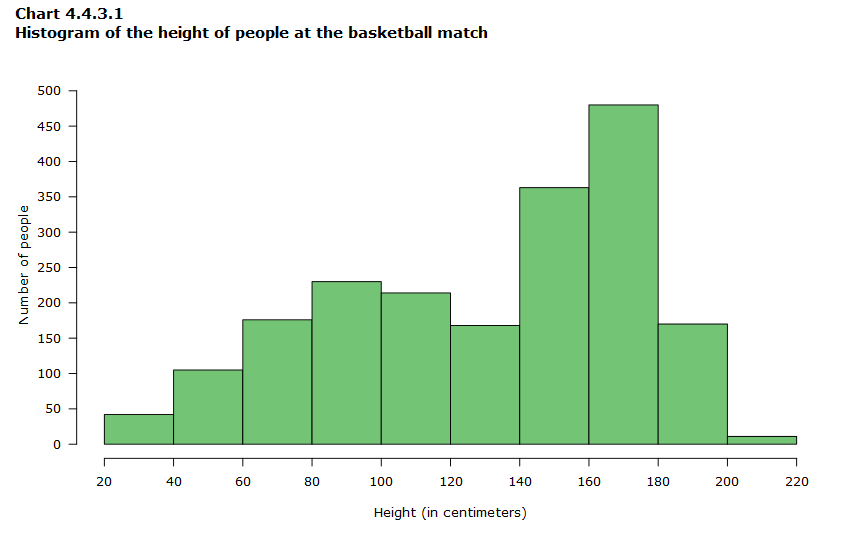
Data table for Chart 4.4.3.1
Data illustrated in this chart are the data from table 4.4.3.5.
Looking at the table and histogram, you can easily identify the modal-class interval, 160 to 179 centimetres, whose frequency is 480. You can also see that as the height decreases from this interval, the frequency also decreases for the interval 140 to 159 centimetres (363) and it continues to decrease for 120 to 139 centimetres (168), before starting to increase until the height reaches 80 to 99 centimetres (230).
For categorical or discrete variables, multiple modes are values that reach the same frequency: the highest one observed. For continuous variables, all peaks of the distribution can be considered modes even if they don’t have the same frequency. The distribution for this example is bimodal, with a major mode corresponding to the modal-class interval 160 to 179 centimetres and a minor mode corresponding to the modal-class interval 80 to 99 centimetres. The modal class shouldn’t be used as a measure of central tendency, but finding two modes gives us an indication that there could be two distinct groups in the data that should be analyzed separately.
- Date modified: